Decision Trees

Decision trees are a popular approach to classification. A decision tree comprises a series of nodes representing “choices” based on some feature of the data. The branches then represent the outcome of this. By following a path through the decision tree, we can predict the class of a given data point.

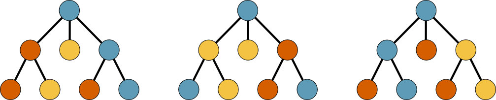
Fig. 28 Three decision trees, where each node is a choice, and the edges are an outcome. The terminal nodes are known as leaves.

One of the advantages of decision trees is that, for many systems, the decision-making process can be understood and interpretable. We should be conscious of the risk of overfitting with decision trees that grow very deep, but some approaches can address this.

Composition of a Decision Tree

The decision tree starts with a root node. This root node splits the data based on the most significant feature present. Following this, several internal nodes test individual features of the data. Finally, the leaf nodes represent the final class prediction, and there are no further splits after these.

The natural question is, how is the data split in each node? The splittings aim to maximise the information gained from the split or minimise the impurity. This is achieved with splitting criteria, such as the Gini impurity, a measure of the likelihood that the classification is incorrect.

Building a Decision Tree

Continuing the practice of other classification approaches, we can create a decision tree algorithm from scratch for the toy data we have been investigating.

import pandas as pd
from sklearn.model_selection import train_test_split

data = pd.read_csv("../data/toy.csv")

data['encoded_label'] = [1 if i == 'b' else 0 for i in data['label'].values]
train, test = train_test_split(data, test_size=0.2, random_state=0)
X = train[['x', 'y']].values
y = train['encoded_label'].values

The first step is to create a function that computes the Gini impurity. The Gini impurity is computed for a given dataset, \(D\), as,

\[ G(D) = 1 = \sum_{i+1}^{C} p_i^2, \]

where \(C\) is the number of classes, and \(p_i\) is the proportion of elements that belong to the class \(i\). Therefore, this can be computed using the function below.

import numpy as np

def gini_impurity(labels):
    """
    Calculate the Gini impurity of a list of labels.
    
    :param y: a list of labels
    
    :return: the Gini impurity of the list
    """
    _, counts = np.unique(labels, return_counts=True)
    p = (counts / labels.size) ** 2
    return 1 - np.sum(p)

If all labels belong to the same class, we have a pure node with a Gini impurity of 0. Let’s compute the Gini impurity for the current training data.

gini_impurity(y)

0.498046875

About 0.5, indicating an even split between the two classes (the data is maximally impure). This is expected as the dataset is 50 % class a and 50 % class b.

The next step is to find the best way to split the data in a given iteration of the training. This is achieved by finding all the potential thresholds for splitting each feature of the data. The data is then split across each of these thresholds, in turn, and the information that is gained (using the Gini impurity) from such a splitting is computed. By iterating through all the thresholds, we can find the best splitting that maximises the information gain.

def find_best_split(X, y):
    """
    Determines the best split for a dataset based
    on the Gini impurity.
    
    :param X: a 2D numpy array of features
    :param y: a 1D numpy array of labels
    
    :return: a tuple of the best feature, best threshold, and best gain
    """
    best_gain = 0
    best_feature = None
    best_threshold = None

    thresholds = np.unique(X, axis=0)
    for feature in range(X.shape[1]):
        for threshold in thresholds:
            y_left = y[np.where(X[:, feature] < threshold[feature])]
            y_right = y[np.where(X[:, feature] >= threshold[feature])]

            weight_left = y_left.size / y.size
            weight_right = y_right.size / y.size
            information_gain = gini_impurity(y) - (weight_left * gini_impurity(y_left) + weight_right * gini_impurity(y_right))

            if information_gain > best_gain:
                best_gain = information_gain
                best_feature = feature
                best_threshold = threshold[feature]

    return best_feature, best_threshold, best_gain

This function will return the index of the best feature to split, the threshold value and how much information will be gained.

find_best_split(X, y)

(0, 1.127395499883415, 0.3150523062047401)

Note

The decision tree provides a really lovely example of recursion, which is an important concept in computer science. In the make_tree function, we call the make_tree function, this is recursion.

Then, to actually use the algorithm, we recursively run through the function below until there is either no information to be gained or no way left to split the data (i.e., we have found all the leaves).

def make_tree(X, y):
    """
    Recursively constructs a decision tree.
    
    :param X: a 2D numpy array of features
    :param y: a 1D numpy array of labels
    
    :returns: a dictionary representing the decision tree
    """
    if len(np.unique(y)) == 1:
        return np.argmax(np.bincount(y))
    
    feature, threshold, gain = find_best_split(X, y)

    if gain == 0:
        return np.argmax(np.bincount(y))

    left_X = X[np.where(X[:, feature] < threshold)]
    left_y = y[np.where(X[:, feature] < threshold)]
    right_X = X[np.where(X[:, feature] >= threshold)]
    right_y = y[np.where(X[:, feature] >= threshold)]

    left_subtree = make_tree(left_X, left_y)
    right_subtree = make_tree(right_X, right_y)

    return {"feature": feature,
            "threshold": threshold, 
            "gain": gain, 
            "left": left_subtree, 
            "right": right_subtree}

tree = make_tree(X, y)

In this implementation, the tree object is a dictionary we can visualise with the plot_tree helper function, which can be downloaded here.

from helper import plot_tree

plot_tree(tree)

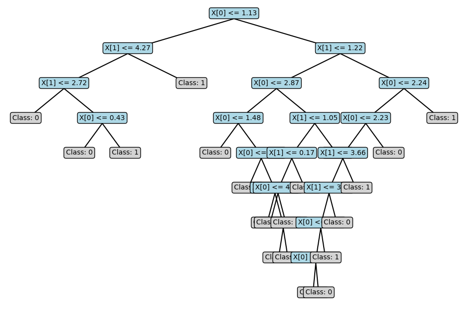
The visualisation isn’t perfect, but you can understand the tree’s structure.

With the tree constructed, predicting from it is simply a matter of traversing the tree for a given sample.

def traverse_tree(x, tree):
    """
    Traverse a decision tree to make a prediction.
    
    :param x: a 1D numpy array of features
    :param tree: a dictionary representing the decision tree
    
    :return: the prediction
    """
    if not isinstance(tree, dict):
        return tree

    feature = tree["feature"]
    threshold = tree["threshold"]

    if x[feature] <= threshold:
        return traverse_tree(x, tree["left"])
    else:
        return traverse_tree(x, tree["right"])
    
traverse_tree(train.iloc[0].values, tree)

0

So, the first value in the training dataset is predicted to be of class a.

Let’s repeat this for all the data points in the training and test datasets to compute our accuracy.

from sklearn.metrics import accuracy_score

prediction = np.array([traverse_tree(x, tree) for x in train[['x', 'y']].values])
prediction_label = np.array(['nd'] * len(prediction))
prediction_label[np.where(prediction == 1)] = 'b'
prediction_label[np.where(prediction == 0)] = 'a'
train['prediction'] = prediction_label

accuracy_score(train['label'], train['prediction'])

0.9

prediction = np.array([traverse_tree(x, tree) for x in test[['x', 'y']].values])
prediction_label = np.array(['nd'] * len(prediction))
prediction_label[np.where(prediction == 1)] = 'b'
prediction_label[np.where(prediction == 0)] = 'a'
test['prediction'] = prediction_label

accuracy_score(test['label'], test['prediction'])

0.95

The decision tree gets a high accuracy for this toy dataset.