Convolutional Layers#
The convolutional layers involve convolving the data with some filter or kernel. This helps to identify spatial features, like edges or textures in images. The concept of convolving data with some kernel may be unfamiliar, so let’s discuss this mathematical operation.
Convolve#
The convolution of two functions, \(f\) and \(g\), is written as \(f * g\). Strictly, this operation is the integral of the product of the two functions after one is reflected about the y-axis and shifted. Graphically, the convolution leads to the shape of one function becoming modified by another. Mathematically, a convolution is written as,
where, \(\tau\) is the shift. Note that convolution is communtative, so \(f * g = g * f\).
Let’s have a look at the convolution of two one-dimensional functions.
import numpy as np
import matplotlib.pyplot as plt
from scipy.stats import norm, uniform

x = np.linspace(-10, 10, 1000)
n = norm.pdf(x)
u =  uniform.pdf(x, loc=-3, scale=6)

fig, ax = plt.subplots()
ax.plot(x, n, label='f(x)')
ax.plot(x, u, label='g(x)')
ax.plot(x, np.convolve(n, u, mode='same') / 20, label='f(x) * g(x) / 20')
ax.set_ylim(0, None)
ax.set_xlabel('x')
ax.legend()
plt.show()
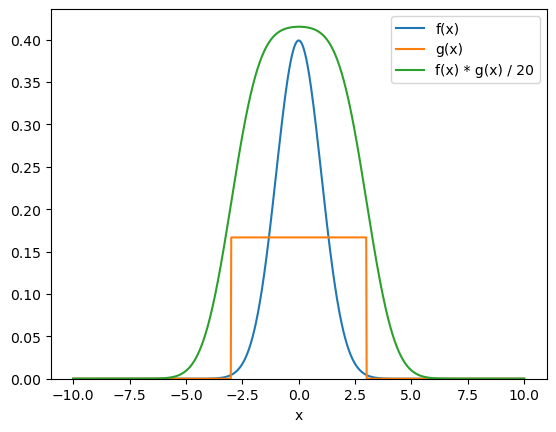
Above, we convolve the standard normal distribution with a uniform distribution to produce a new distribution with the character of both.
Note that the mode is set to 'same', such that the output is on the same scale as the maximum from the inputs.
The way that a convolution works can be seen in the following animation.
Fig. 40 A gif showing the process of convolving a uniform distribution with an impulse response. Reproduced under a CC BY-SA 3.0 license.#
The convolution is closely related to the cross-correlation, with the only difference being that the cross-correlation function does not reflect either function in the y-axis.
Image Convolution#
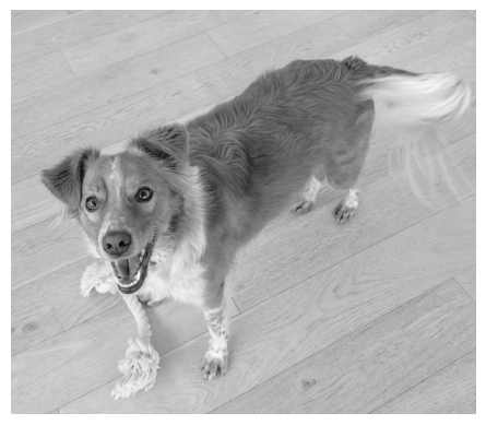
Convolutional neural networks are commonly applied to image classification problems. This means that the convolutions are being applied over the two dimensions of the image. Let’s see the result of one such convolutional filter on an image of a very cute dog.
pepe = np.loadtxt('../data/pepe.txt')

fig, ax = plt.subplots()

ax.imshow(pepe, cmap='gray')
ax.axis('off')
plt.show()
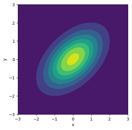
For this, we will apply a Gaussian filter with x and y means of 0 and the following covariance matrix.
means = [0, 0]
cov = [[1, 0.5], [0.5, 1]]
We will construct the Gaussian filter using the scipy.stats.multivariate_normal object.
from scipy.stats import multivariate_normal

mv = multivariate_normal(means, cov)
And visiualise this distribution with a contour plot.
x, y = np.mgrid[-3:3:.01, -3:3:.01]

fig, ax = plt.subplots()

ax.contourf(mv.pdf(np.dstack((x, y))), extent=(-3, 3, -3, 3))
ax.set_aspect('equal')
ax.set_xlabel('x')
ax.set_ylabel('y')
plt.show()
Above, we have used a very fine grid over which the PDF has been computed. However, in the convolution context, the convolutional kernel’s size is also important. Here, we will use a 30×30 convolutional filter to show the effect.
kernel = mv.pdf(np.dstack(np.mgrid[-3:3:.2, -3:3:.2]))
kernel.shape
(30, 30)
To perform this convolution, we use the scipy.signal.convolve2d function, again with the mode as 'same'.
from scipy.signal import convolve2d

pepe_convolved = convolve2d(pepe, kernel, mode='same')

fig, ax = plt.subplots(1, 2, figsize=(10, 5))

ax[0].imshow(pepe, cmap='gray')
ax[1].imshow(pepe_convolved, cmap='gray')
ax[0].axis('off')
ax[1].axis('off')
ax[0].set_title('Original')
ax[1].set_title('Convolved')
plt.show()
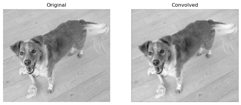
From passing the convolutional filter over the image, we get a more smeared-out version of the image. This is known as a Gaussian blur kernel. This is not the only type of filter that exists. Indeed, different filters serve different purposes in image classification. For example, the Prewitt and Sobel filters are popular for edge detection.
Changing Filters#
During the training of a neural network, the filters are among the trained parameters. This means that the analysis of the filters in a network can be informative about the trends being discovered. By investigating the filters trained in the network, we can begin to understand what the network has learnt.