Logistic Regression#
Logistic regression is confusingly named because it is used for binary classification, not regression. It is called regression, as a regression model describes the relationship between the input features and the probability of a specific outcome. To get started, look at the logistic function, which sits at the heart of the logistic regression algorithm.
Logistic Function#
The logistic function is a type of sigmoid function that can be used in any area of mathematics,
where \(z\) is the input variable. Let’s plot the logistic function.
import numpy as np
import matplotlib.pyplot as plt

def logistic(z):
    """
    Compute the logistic function
    :param z: input

    :return: output of the logistic function
    """
    return 1 / (1 + np.exp(-z))

z = np.linspace(-10, 10, 100)
logistic_z = logistic(z)

fig, ax = plt.subplots()
ax.plot(z, logistic_z)
ax.set_xlabel('z')
ax.set_ylabel('logistic(z)')
plt.show()
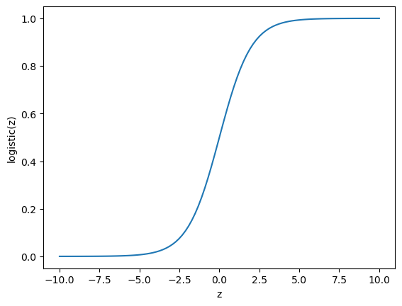
It is clear that the logistic function can only have values of between 0 and 1. This enables binary classification, where one class is associated with the value 0, and the other is associated with the value 1. Therefore, if the value of z (we will come to how z is calculated in a bit) is 7.5, the logistic function has a value of:
logistic(7.5)
0.9994472213630764
Clearly, this would be of class 1. However, what if the value of z is 0.1?
logistic(0.1)
0.52497918747894
In this case, we round using rounding half-up rules. So this would also be of class 1.
The logistic function (and other sigmoidal functions) is extremely important in binary classification approaches. These can be generalised to classify \(N\) classes using softmax regression (multinomial logistic regression).
Softmax Regression#
Softmax regression uses a multinomial (multidimensional) logistic probability distribution with the following form,
where \(\mathbf{z}\) is a vector of length \(K\), and each vector member is associated with a class \(j\). So if there are three classes, a, b, and c, for which the vector \(\mathbf{z}\) is:
z = np.array([2.0, 1.0, 0.5])
We can compute the softmax function using scipy.
from scipy.special import softmax

softmax(z)
array([0.62853172, 0.2312239 , 0.14024438])
We see that the vector \(\mathbf{z}\) has the following probabilities for each class, given the vector \(\mathbf{z}\):
\(P(a|\mathbf{z}) = 62.9\%\)
\(P(b|\mathbf{z}) = 23.1\%\)
\(P(c|\mathbf{z}) = 14.0\%\)
So, the vector \(\mathbf{z}\) is most likely to describe something in class a. Using a logistic function means a probability can be associated with the classification, which is impossible for all classification algorithms.
Linear Combination#
The input to the logistic function is found from a linear combination of our input features, \(\mathbf{x}\). Each of these input features is weighted; we can think of these weights \(\mathbf{w}\), as how important they are in the classification, and finally, a bias term, \(b\), is added, giving,
where \(N\) is the features in the data. We can also write this function as a dot product,
We optimise these weights and bias terms in the training part of our machine-learning workflow.
Optimisation#
Typically, gradient descent or similar algorithms are used to optimise the values of the weights and bias. This leads to another common term from the machine learning world, learning rate. Since we are using gradient descent, a step size for the optimisation must be defined. This is the learning rate.
The final thing to consider is what we are optimising. This is called the loss function of the algorithm; a common loss function for logistic regression is the cross-entropy loss,
where the summation is over the \(m\) training data points, each with the value \(y_i\), and \(f(z_i)\) is the model result using the logistic function discussed above. Let’s look at applying logistic regression to some example datasets.