Singular Value Decomposition#
Singular Value Decomposition (or SVD) is a generalisation of eigendecomposition that breaks any shape of a matrix down to simpler components. So, while eigendecomposition requires the input matrix to be square, SVD does not have this expectation. The SVD of the matrix \(\mathbf{A}\) can be written as:
The components that SVD decomposes \(\mathbf{A}\) can be considered the application of three individual linear transformations, shown in Fig. 17.
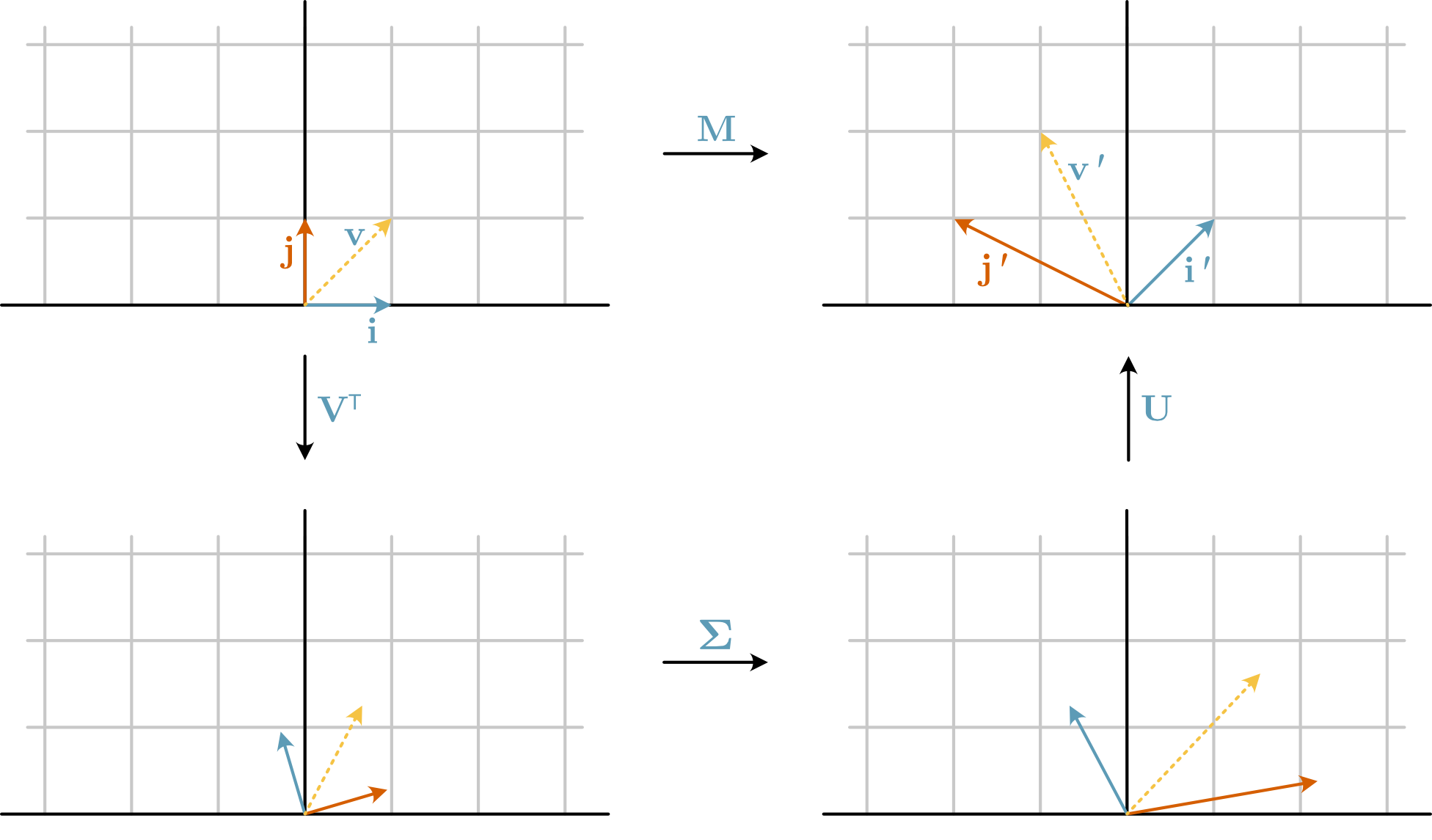
Fig. 17 The decomposition of the matrix \(\mathbf{M}\) into \(\mathbf{V}^\top\), \(\mathbf{\Sigma}\), and \(\mathbf{U}\).#
These linear transformations perform the following geometrical operations to the vector space:
\(\mathbf{V}^\top\): Rotates the input space.
\(\mathbf{\Sigma}\): Stretches the rotated space along the principal axes by factors given by the singular values, \(\mathbf{S}\).
\(\mathbf{U}\): Rotates the new stretched space.
SVD in NumPy#
NumPy can be used to perform SVD for a given matrix. Consider the matrix \(\mathbf{M}\) in Fig. 17 above, which has the value,
We can find the SVD components using NumPy, which is as follows:
import numpy as np

M = np.array([[-2, 1], [1, 1]])
U, S, Vt = np.linalg.svd(M)
We can numerically check the observed transformation of the vector \(\mathbf{v}\).
v = np.array([[1], [1]])
Let’s start with the rotation by \(\mathbf{V}^\top\).
Vt @ v
array([[0.66730788],
       [1.24687618]])
This new position agrees well with the observed rotation in Fig. 17. Next, we add the stretching using \(\mathbf{\Sigma}\), a diagonal matrix with diagonal values of \(\mathbf{S}\).
np.diag(S) @ Vt @ v
array([[1.53666032],
       [1.6243999 ]])
Finally, to reach the vector of \(\mathbf{v}' = -1 \mathbf{i} + 2 \mathbf{j}\), we rotate by \(\mathbf{U}\).
U @ np.diag(S) @ Vt @ v
array([[-1.],
       [ 2.]])
This gives us the expected outcome.
How To Perform SVD?#
The individual components from SVD can be described as follows:
\(\mathbf{U}\): The columns of \(\mathbf{U}\) are the eigenvectors of the matrix \(\mathbf{M}\mathbf{M}^\top\).
\(\mathbf{\Sigma}\): Represent the “strength” of each mode in the transformation and is a diagonal matrix, where the diagonal values are the square roots of the eigenvalues of \(\mathbf{M}^\top\mathbf{M}\).
\(\mathbf{V}^\top\): The columns of \(\mathbf{V}\) are the eigenvectors of the matrix \(\mathbf{M}^\top\mathbf{M}\).
Let’s check these, starting with \(\mathbf{U}\).
np.linalg.eig(M @ M.T).eigenvectors, U
(array([[ 0.95709203,  0.28978415],
        [-0.28978415,  0.95709203]]),
 array([[-0.95709203,  0.28978415],
        [ 0.28978415,  0.95709203]]))
These values are the same, accounting for some numerical sign-switching. This sign switching is simply a 180 ° rotation of the vector space, which arrives because SVD is not unique.
We can now look at \(\mathbf{\Sigma}\).
np.sqrt(np.linalg.eig(M.T @ M).eigenvalues), S
(array([2.30277564, 1.30277564]), array([2.30277564, 1.30277564]))
The np.linalg.svd algorithm sorts S so that the largest value is first.
The algorithm does the same to the \(\mathbf{V}^\top\) matrix; therefore, to get agreement, the columns need to be sorted.
cols = np.argsort(np.linalg.eig(M.T @ M).eigenvalues)[::-1]
np.linalg.eig(M.T @ M).eigenvectors[:, cols], Vt
(array([[ 0.95709203,  0.28978415],
        [-0.28978415,  0.95709203]]),
 array([[ 0.95709203, -0.28978415],
        [ 0.28978415,  0.95709203]]))
Again, the values agree, accounting for the non-unique nature of singular value decomposition.