Matrices

Following on from vectors, another mathematical object that may be familiar is matrices. A matrix is an array of numbers, indeed, it is possible to think of a vector as a one-dimensional matrix. Matrices are extremely important across a wide range of mathematical topics — here they will be used to represent linear transformations.

Matrices are rectangular and contain several values, e.g.,

(13)\[\begin{split} \mathbf{A} = \begin{bmatrix} 2 & 4 & 1 \\ 4 & 3 & 7 \end{bmatrix}, \end{split}\]

which would be referred to as a 2×3 matrix, as there are 2 rows and 3 columns. Commonly matrix elements are indexed by their row and column, i.e., in \(\mathbf{A}\) one may write that \(a_{13}\) has the value of 1. Hence, the notation for an arbitrary matrix of

(14)\[\begin{split} \mathbf{A} = \begin{bmatrix} a_{11} & a_{12} & \cdots & a_{1n} \\ a_{11} & a_{12} & \cdots & a_{1n} \\ \vdots & \vdots & \ddots & \vdots \\ a_{m1} & a_{m2} & \cdots & a_{mn} \end{bmatrix}. \end{split}\]

Matrix Transpose

The transposition of a matrix is an important operation, however, the physical interpretation of it is complex and beyond the scope of this course. Instead, a visual interpretation can be considered, where the transpose of a matrix is thought of as swapping columns for rows in the matrix, i.e., every column becomes a row and every row a column. This means that for some matrix, \(\mathbf{A}\) that has 5 rows and 3 columns, the transpose, \(\mathbf{A}^\top\), which has 3 rows and 5 columns. Within the concept of handling data, matrix transposes can be particularly valuable, for example, if a particular function requires data to be as columns, but it is provided as rows. Transposing a matrix can be thought of as drawing an imaginary line along the first diagonal and rotating the values of the matrices around this.

Fig. 13 A visual description of a matrix transpose.

Basis Set of Vectors as a Matrix

The standard basis set of vectors, shown in Fig. 11 and defined in Eqn. (9) can be written as a single matrix, where the first column is the \(\mathbf{i}\) column vector and the second is the \(\mathbf{j}\) column vector. This results in the vector \(\mathbf{M}\),

(15)\[\begin{split} \mathbf{M} = \begin{bmatrix} 1 & 0 \\ 0 & 1 \end{bmatrix}, \end{split}\]

which may be familiar to some as an identity matrix, a square matrix with values of one along the diagonal and values of zero elsewhere.

Now, consider the new basis set of vectors that were introduced in Fig. 12, these can be written as the matrix, \(\mathbf{M'}\),

(16)\[\begin{split} \mathbf{M'} = \begin{bmatrix} 0 & -1 \\ 1 & 0 \end{bmatrix}. \end{split}\]

The new basis set of vectors was previously shown to perform a linear transformation of the vector \(\mathbf{r}\). This can also be acheived using the matrix \(\mathbf{M'}\) with matrix multiplication,

(17)\[\begin{split} \mathbf{r'} = \mathbf{M'}\mathbf{r} = \begin{bmatrix} 0 & -1 \\ 1 & 0 \end{bmatrix} \begin{bmatrix} 2 \\ 3 \end{bmatrix} = \begin{bmatrix} -3 \\ 2 \end{bmatrix} \end{split}\]

This vector can also be written as \(-3\mathbf{i} + 2\mathbf{j}\), as in Eqn. (11).

Matrix Multiplication

Matrix multiplication may not be familiar to everyone therefore, we will discuss it using the concept of algorithmic thinking to break down the complexity. Note, that we can use NumPy to perform matrix multiplication but it is valuable to know what the process is. However, you may want to think of this page as a reference, as it can be easy to forgot the algorithm.

Consider the requirement to multiply two matrices, for example;

(18)\[\begin{split}\mathbf{A} = \begin{bmatrix} 4 & 1 \\ 5 & 3 \\ 1 & 2 \\ 2 & 2 \end{bmatrix} \;\;\;\;\;\;\;\;\; \mathbf{B} = \begin{bmatrix} 2 & 1 & 3 \\ 2 & 5 & 1 \end{bmatrix}.\end{split}\]

However, the algorithm should be general, therefore the matrices can be written in general terms

(19)\[\begin{split}\mathbf{A} = \begin{bmatrix} a_{11} & a_{12} \\ a_{21} & a_{22} \\ a_{31} & a_{32} \\ a_{41} & a_{42} \end{bmatrix} \;\;\;\;\;\;\;\;\; \mathbf{B} = \begin{bmatrix} b_{11} & b_{12} & b_{13} \\ b_{21} & b_{22} & b_{23} \end{bmatrix},\end{split}\]

where the symbols in Eqn. (19) may be swapped for the numbers in Eqn. (18) (or any other matrix).

The leading matrix, \(\mathbf{A}\), has the shape 4 × 2 and the trailing, \(\mathbf{B}\), has the shape 2 × 3. The number of columns in the first matrix must be equal to the number of rows in the second and therefore, these matrices can be multiplied.

The resulting matrix, \(\mathbf{C}\), will have the shape: number of rows in the leading matrix × number of columns in the trailing matrix. Therefore, \(\mathbf{C}\) will have the shape 4 × 3, which can be written generally as

(20)\[\begin{split}\mathbf{C} = \begin{bmatrix} c_{11} & c_{12} & c_{13} \\ c_{21} & c_{22} & c_{23} \\ c_{31} & c_{32} & c_{33} \\ c_{41} & c_{42} & c_{43} \end{bmatrix}\end{split}\]

Then starting with \(c_{11}\), this is calculated as the sum of the pairwise product of the matching row in \(\mathbf{A}\) and the matching column in \(\mathbf{B}\), i.e., \(c_{11} = a_{11} b_{11} + a_{12} b_{21}\). Next \(c_{12}\) and \(c_{13}\) are found with the same process.

Once we reach the end of the row, the next row is computed \(c_{21}\), \(c_{22}\), etc. and this process continues until all of the values in \(\mathbf{C}\) have been filled.

Fig. 14 A schematic diagram of matrix multiplication. Source: Wikipedia/Matrix multiplication

Inverse of a Matrix

Thinking about matrices in terms of linear transformations gives a physical interpretation to the matrix inverse, i.e., that it is the opposite linear mapping operation. For a 2×2 matrix, the inverse, which is indicated with the superscript \(-1\), can be found easily by hand,

(21)\[\begin{split} \begin{bmatrix} a & b \\ c & d \end{bmatrix}^{-1} = \frac{1}{ad-bc} \begin{bmatrix} d & -b \\ -c & a \end{bmatrix}, \end{split}\]

where \(ad-bc\) is the matrix determinant. The larger the matrix, the more complex the inverse is to calculate by hand but it is possible to use NumPy to make that easier. Be aware, that it is only possible to calculate the inverse of a square matrix, i.e., where the number of rows and columns are the same.

The Matrix Determinant

The determinant of a matrix is a scalar value that exists for square matrices. There is no such thing as a determinant of a rectangular matrix, leading to the fact that rectangular matrices are not invertible.

There is a geometric interpretation of the determinant of a matrix that builds on the understanding of matrices as linear transformations. The determinant of a matrix is the area of the parallelogram that represents the unit square of the new basis set of vectors in the standard basis set of vectors. This is more straightforward to consider with an example.

Consider the 2×2 matrix \(\mathbf{A}\),

(22)\[\begin{split} \mathbf{A} = \begin{bmatrix} 1 & -1 \\ 1 & 2 \end{bmatrix}. \end{split}\]

This matrix defines the new basis set of vectors and the unit square is the square that is formed by adding the vector \(\mathbf{j'}\) to \(\mathbf{i'}\) and vice versa, shown in Fig. 15. The determinant is then the area of this unit square.

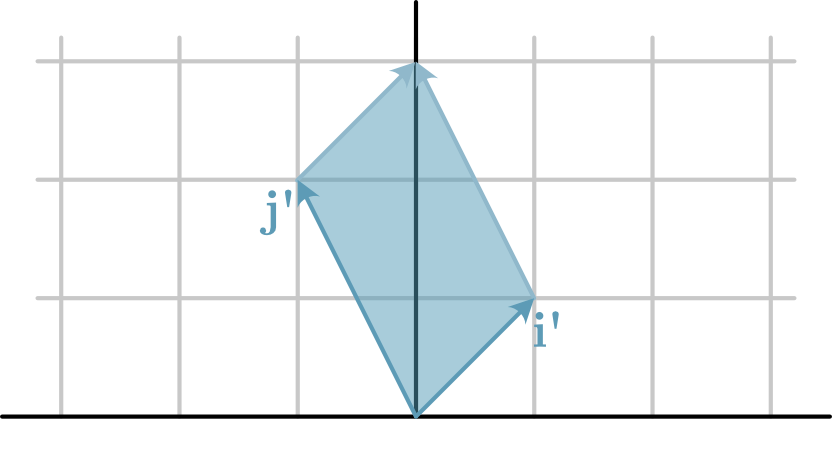
Fig. 15 The new basis set, defined by \(\mathbf{A}\), showing the unit square (shaded blue), which the determinant is the area of.

For a general 2×2 matrix, \(\mathbf{X}\), where

(23)\[\begin{split} \mathbf{X} = \begin{bmatrix} a & b \\ c & d \end{bmatrix}. \end{split}\]

The determinant is calculated as,

(24)\[ \mathrm{det}(\mathbf{X}) = ad - bc. \]

Therefore for the matrix \(\mathbf{A}\) above, the determinant is \(1\times2 - (1 \times - 1) = 2 + 1 = 3\). This can be confirmed visually by counting the squares that the blue shaded region covers in Fig. 15.