Build Your Own GMM

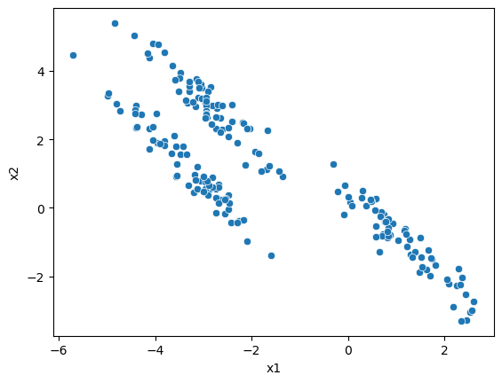
To look at the Gaussian mixture models algorithm, let’s use the same data that caused problems for k-means previously.

import numpy as np
import pandas as pd
import seaborn as sns
import matplotlib.pyplot as plt
from sklearn import datasets

data = pd.read_csv('../data/skew.csv')

fig, ax = plt.subplots()
sns.scatterplot(x='x1', y='x2', data=data, ax=ax)
plt.show()

It is common practice to start the GMM algorithm from an estimate of the cluster centres, for example, from k-means clustering. We assign these centres to the Gaussian mixture model’s means, \(\mu_k\).

from sklearn.cluster import KMeans

means = KMeans(n_clusters=3).fit(data).cluster_centers_
means

array([[-2.61539758,  0.6116586 ],
       [ 1.19011929, -1.04498941],
       [-3.38180527,  3.01284449]])

We can see that the three mean values are two-dimensional; luckily, there is a scipy.stats object that describes an N-dimensional Gaussian distribution. This is called scipy.stats.multivariate_normal; let’s look at the documentation for this object.

from scipy.stats import multivariate_normal

multivariate_normal?

We can see that it takes means and a covariance matrix, the latter is, for a two-dimensional distribution, a 2×2 matrix. A good starting point for this matrix would be the covariance matrix of the data.

covs = np.array([np.cov(data.T) for i in range(3)])
covs

array([[[ 4.66253907, -3.53992547],
        [-3.53992547,  3.75965887]],

       [[ 4.66253907, -3.53992547],
        [-3.53992547,  3.75965887]],

       [[ 4.66253907, -3.53992547],
        [-3.53992547,  3.75965887]]])

We can now create the three two-dimensional Gaussian distributions that we will use to describe the data.

mvs = [multivariate_normal(mean=mean, cov=cov) for mean, cov in zip(means, covs)]

And we can plot them alongside the data.

x1 = np.linspace(data['x1'].min(), data['x1'].max(), 1000)
x2 = np.linspace(data['x2'].min(), data['x2'].max(), 1000)

X1, X2 = np.meshgrid(x1, x2)

fig, ax = plt.subplots(1, 3, figsize=(15, 4))

for i, ax in enumerate(ax):
    ax.contour(X1, X2, mvs[i].pdf(np.dstack((X1, X2))), cmap='Grays')
    ax.scatter(data['x1'], data['x2'])
    ax.set_title(f'Cluster {i}')
    ax.set_xlabel('x1')
    ax.set_ylabel('x2')
plt.show()

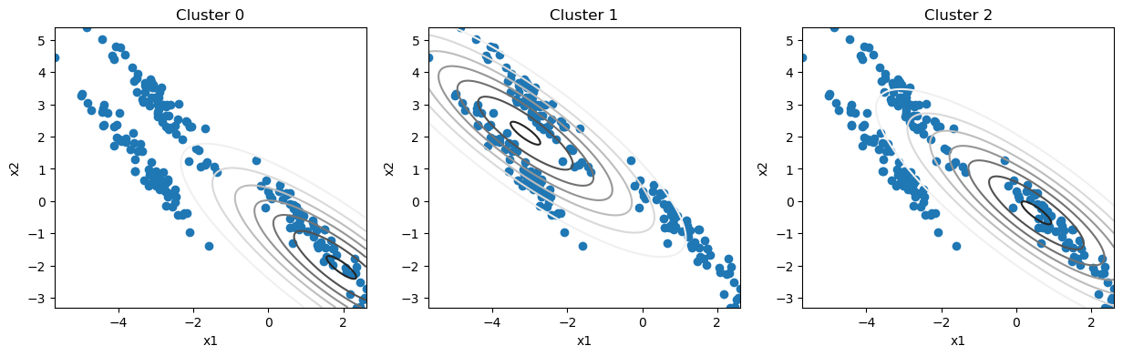
This is not a very good estimate of the clusters. But, we can use the EM algorithm of Gaussian mixture models to improve the estimates.

First, let’s look at computing the responsibilities, the responsibility, \(\gamma_{i, k}\) of a given data point, \(x_i\), for Gaussian distribution \(k\), where \(k \in K\), is computed as,

\[ \gamma_{i, k} = \frac{\pi_k \mathcal{N}(x_i | \mu_k, \Sigma_k)}{\sum_{j=1}^{K}\left[\pi_j \mathcal{N}(x_i | \mu_j, \Sigma_j)\right]}, \]

where \(\pi_k\) is the weight of cluster \(k\) (all the weights should sum to 1), and we read \(\mathcal{N}(x_i | \mu_k, \Sigma_k)\) as the probability of \(x_i\) given the normal distribution \(\mathcal{N}(\mu_k, \Sigma_k)\). This can be thought of as the probability of finding a given data point in a given normal distribution. We can write code to achieve this expectation step.

def expectation(data, mvs, weights):
    """
    Computate the responsibility for the data points given the current cluster MVs. 
    
    :param data: The data points.
    :param mvs: The cluster MVs.
    :param weights: The weights of the clusters.
    
    :return: The responsibilities for the data points.
    """
    responsiblities = np.zeros((data.shape[0], len(mvs)))
    for i, mv in enumerate(mvs):
        responsiblities[:, i] = weights[i] * mv.pdf(data)
    responsiblities /= responsiblities.sum(axis=1)[:, np.newaxis]
    return responsiblities

With the responsibilities calculated, it is time to update the parameters: the means, covariance matrices and weights. This is achieved in the maximisation step.

The mean for cluster \(k\) is computed as the sum of the product of the responsibilities, and the data is divided by the sum of the responsibilities.

\[ \mu_k = \frac{\sum_{i=1}^{N}\left(\gamma_{i, k} x_i\right)}{\sum_{i=1}^{N}\left(\gamma_{i, k}\right)}. \]

Note

Be aware that this implementation of the new_means function is vectorised to perform it for all \(K\) clusters in a single operation.

def means_update(responsiblities, data):
    """
    Compute the new means given the responsibilities and the data points.
    
    :param responsiblities: The responsibilities for the data points.
    :param data: The data points.
    
    :return: The new means.
    """
    return np.dot(responsiblities.T, data) / responsiblities.sum(axis=0)[:, np.newaxis]

The new covariances are computed with the difference between the data and the updated mean positions,

\[ \Sigma_k = \frac{\sum_{i=1}^{N}\left\{\left[\gamma_{i,k}(x_i - \mu_k)\right]^\top(x_i - \mu_k)\right\}}{\sum_{i=1}^{N}\left(\gamma_{i, k}\right)}. \]

Again, we can write this in Python as,

def covariances_update(responsiblities, data, means):
    """
    Compute the new covariances given the responsibilities, data points, and means.
    
    :param responsiblities: The responsibilities for the data points.
    :param data: The data points.
    :param means: The means of the clusters.
    
    :return: The new covariances.
    """
    covs = np.zeros((len(means), data.shape[1], data.shape[1]))
    for i in range(responsiblities.shape[1]):
        diff = data - means[i]
        covs[i] = np.dot((responsiblities[:, i][:, np.newaxis] * diff).T, diff) / responsiblities[:, i].sum()
    return covs

Finally, the new weights are found as the average of the responsibilities,

\[ \mu_k = \frac{\sum_{i=1}^{N}\gamma_{i, k}}{N}. \]

def weights_update(responsiblities):
    """
    Compute the new weights given the responsibilities.
    
    :param responsiblities: The responsibilities for the data points.
    
    :return: The new weights.
    """
    return responsiblities.mean(axis=0)

We can put this together in a loop, with initial weights of one-third each.

weights = np.ones(3) / 3

for i in range(3):
    responsiblities = expectation(data.values, mvs, weights)
    means = means_update(responsiblities, data.values)
    covs = covariances_update(responsiblities, data.values, means)
    weights = weights_update(responsiblities)
    mvs = [multivariate_normal(mean=mean, cov=cov) for mean, cov in zip(means, covs)]

After three iterations of the algorithm, let’s see how the distributions look.

fig, ax = plt.subplots(1, 3, figsize=(15, 4))

for i, ax in enumerate(ax):
    ax.contour(X1, X2, mvs[i].pdf(np.dstack((X1, X2))), cmap='Grays')
    ax.scatter(data['x1'], data['x2'])
    ax.set_title(f'Cluster {i}')
    ax.set_xlabel('x1')
    ax.set_ylabel('x2')
plt.show()

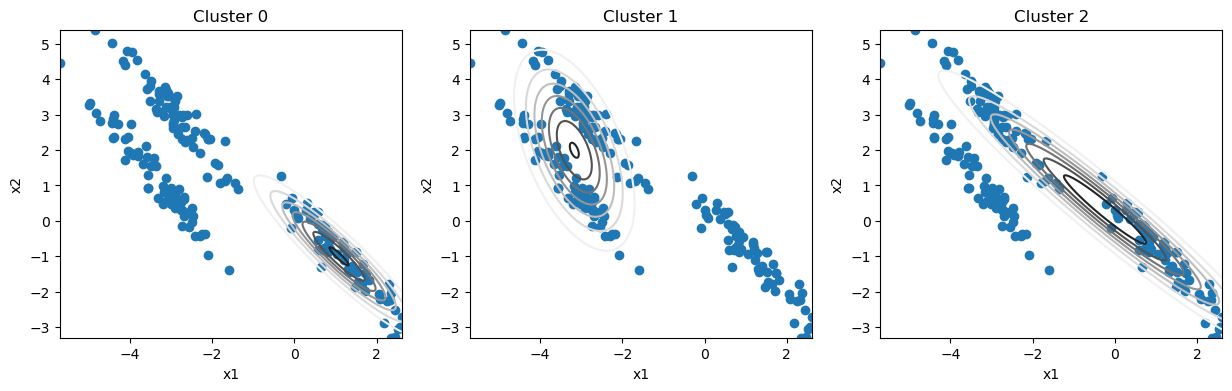
We can see that even after a small number of iterations, we describe the clusters well. Now, we will introduce a convergence criteria that will stop the iterative process. In this case, we will choose the point when the parameters stop changing.

means_list = [means]
covs_list = [covs]
weights_list = [weights]

for i in range(100):
    responsiblities = expectation(data.values, mvs, weights)
    means_list.append(means_update(responsiblities, data.values))
    covs_list.append(covariances_update(responsiblities, data.values, means_list[-1]))
    weights_list.append(weights_update(responsiblities))
    mvs = [multivariate_normal(mean=mean, cov=cov) for mean, cov in zip(means_list[-1], covs_list[-1])]
    if np.allclose(means_list[-1], means_list[-2]) and np.allclose(covs_list[-1], covs_list[-2]) and np.allclose(weights_list[-1], weights_list[-2]):
        break
print(f'Stopped after {i} iterations')

Stopped after 7 iterations

Only an additional seven iterations were necessary for convergence.

fig, ax = plt.subplots(1, 3, figsize=(15, 4))

for i, ax in enumerate(ax):
    ax.contour(X1, X2, mvs[i].pdf(np.dstack((X1, X2))), cmap='Grays')
    ax.scatter(data['x1'], data['x2'])
    ax.set_title(f'Cluster {i}')
    ax.set_xlabel('x1')
    ax.set_ylabel('x2')
plt.show()

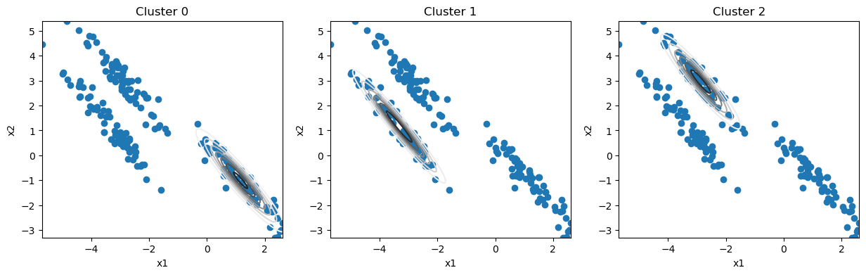
From this, we can generate cluster labels for each data point. The cluster with the highest responsibility for a given data point is the one to which the data point is assigned. We can find this with the np.argmax function.

cluster_labels = np.argmax(responsiblities, axis=1)

data_label = data.copy()
data_label['labels'] = cluster_labels
fig, ax = plt.subplots()
sns.scatterplot(x='x1', y='x2', data=data_label, hue='labels', ax=ax)
plt.show()

We can treat the responsibilities of each data point for each cluster as a probability. This probability describes how likely the data point is associated with a given cluster. This means that we can visualise the probability that a data point is a member of a cluster with the size of the marker.

size = 10 * responsiblities.max(axis=1) ** 2

fig, ax = plt.subplots()
ax.scatter(data['x1'], data['x2'], c=cluster_labels, s=size)
plt.show()

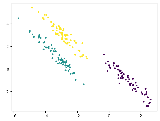
It is clear that the points closer to the centre of each distribution, where the probability density function is greater, are more likely to be members of a given cluster.