Vector Operations#
The complexity of Fig. 7 is reduced slightly in Fig. 8 by showing only the vectors.
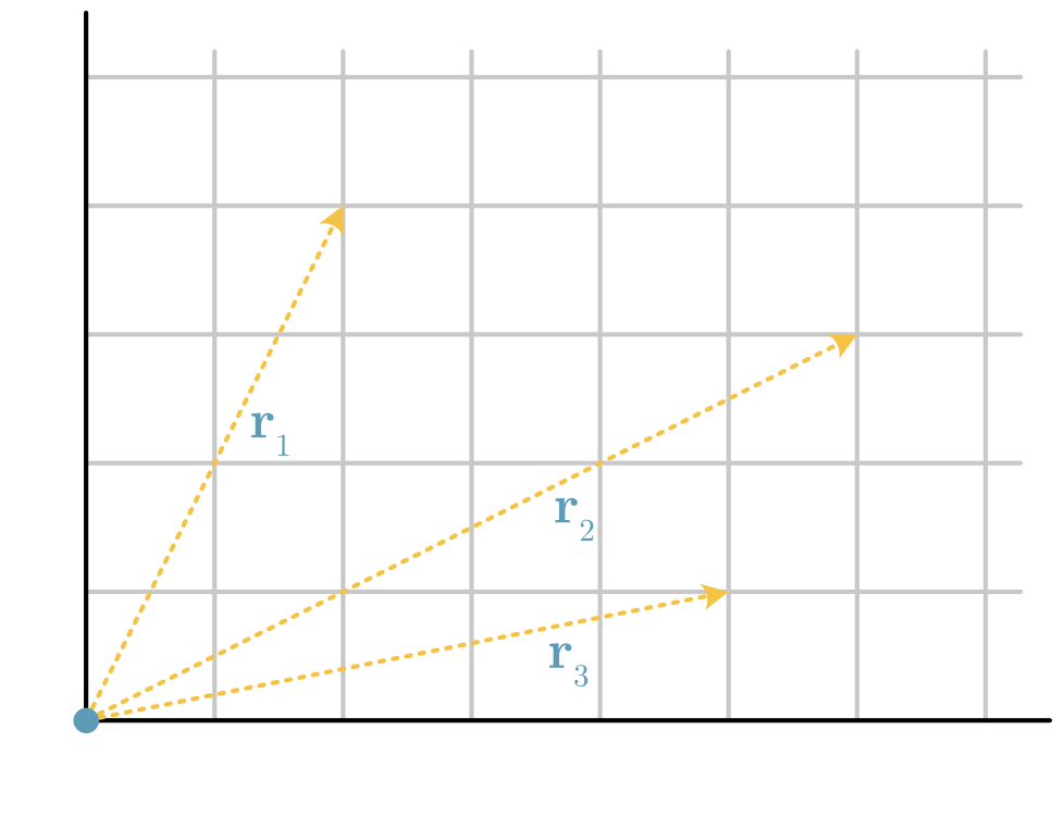
Fig. 8 The vector-only description of the particle positions.#
Vector arithmetic#
Now it is possible to consider what happens when arithmetic is performed between two vectors. Consider the vector between particle 1 and 2, \(\mathbf{r}_{12}\) (Fig. 9), which can be found via vector subtraction, e.g.,
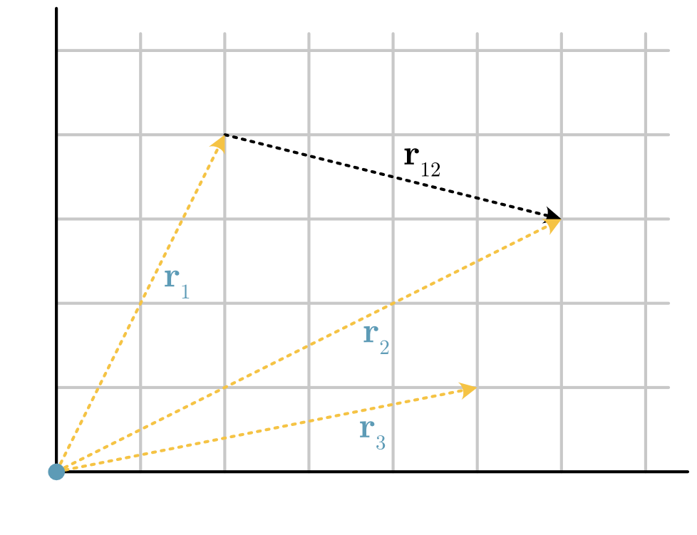
Fig. 9 The result of vector subtraction to determine the vector between two points.#
This is the difference between the common terms for the basis vectors,
From this, the magnitude of the vector (the length) can be computed, which is the distance between particles 1 and 2. This is the root sum of squares for the individual components, i.e., the magnitude of \(\mathbf{r}_{12}\) is,
Similar to traditional subtraction and addition, we can rearrange Eqn. (3) to give vector addition,
So if the vectors \(\mathbf{r}_1\) and \(\mathbf{r}_{12}\) are known it is possible to calculate the vector \(\mathbf{r}_2\).
The dot product#
The dot product is a type of vector multiplication that returns a single value, hence it can be referred to as the scalar product (to distinguish from the vector, cross product). The mathematical operation for the dot product, written as \(\mathbf{a} \cdot \mathbf{b}\), the sum of the product of the individual components of each vector, i.e.,
The dot product has the additional utility that it can be used to calculate the angle between the two vectors, \(\theta\), using the alternative definition
where the \(|\mathbf{a}|\) indicates the magnitude of the vector \(\mathbf{a}\)
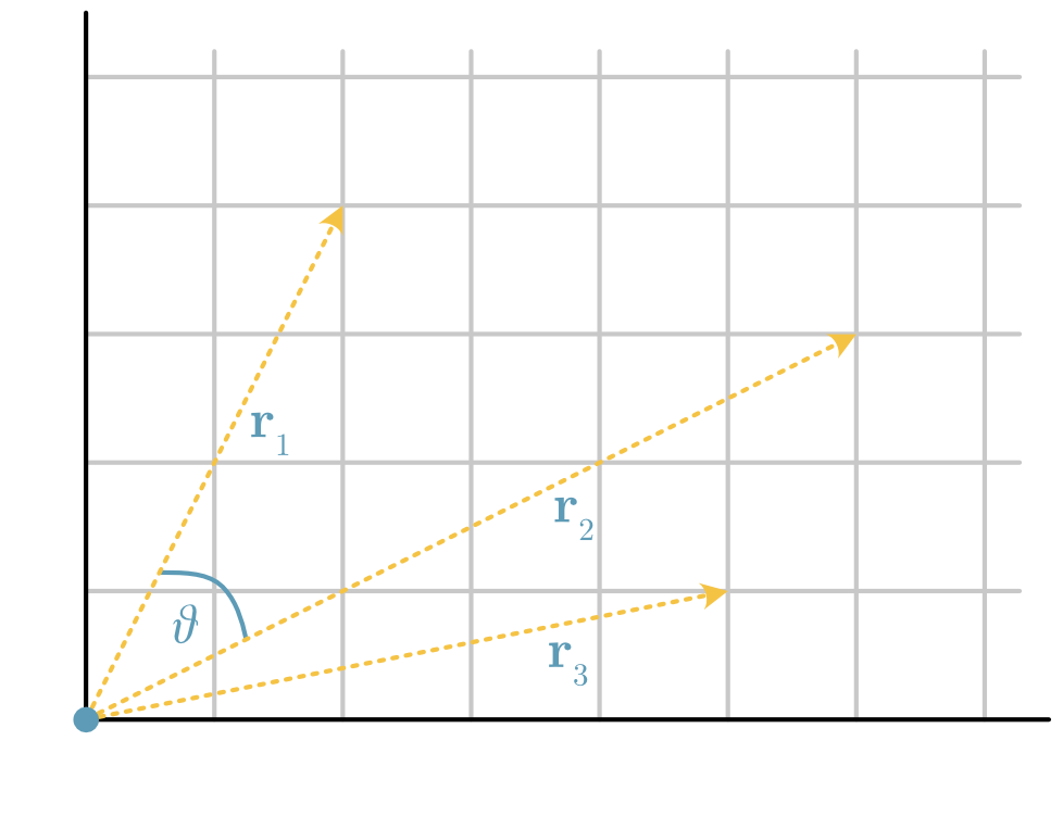
Fig. 10 The angle, \(\theta\), between two vectors.#
Vector with NumPy#
Consider again the vectors in Fig. 8, we can define NumPy arrays that describe these.
import numpy as np

r1 = np.array([2, 4])
r2 = np.array([6, 3])
r3 = np.array([5, 1])
In addition to thinking of these arrays as arrays of data, as is typically the case for NumPy, we can also think of these as our vectors. NumPy arrays lend themselves naturally to vector arithmetic operations, like subtraction.
r12 = r2 - r1
print(r12)
[ 4 -1]
Converting vectors to arrays
Above, NumPy arrays are used to represent mathematical vectors.
However, it is sometimes desirable to increase the dimensionality of a vector, turning from a one-dimensional NumPy array to a two-dimensional row or column matrix.
This can be achieved with either the reshape() method or by using the np.newaxis keyword in conjunction with a slicing operation.
For example, r1 has the value,
array([2, 4])
While, r1.reshape(-1, 1) and r1[:, np.newaxis] have the value,
array([[2],
       [4]])
The -1 in the reshape method tells it to use a value that will work with the other value, in this case, the 1 that follows.
This is because it is only possible to reshape into shapes that the original NumPy array will fit.
This reshaping operation can be very useful in allowing the efficiency of NumPy to be leveraged. Often removing the need to perform a loop over a series of NumPy arrays, simply by restructuring the problem.
Notice that this is the same result as found previously in Eqn. (4). There is even a convenient function to find the magnitude of a vector, also known as the vector norm.
d12 = np.linalg.norm(r12)
print(d12)
4.123105625617661
Additionally, the dot product between two vectors can be found in two ways.
dot_product = np.dot(r1, r2)
print(dot_product)
24
times_and_sum = np.sum(r1 * r2)
print(times_and_sum)
24
Notice that both approaches produce the same result.