t-SNE

t-distributed stochastic neighbour embedding or t-SNE is another dimensionality reduction algorithm. The use case for t-SNE is different from PCA in that it is strongly focused on the visualisation of data, and the interpretability of the t-SNE model is usually very low. However, the nature of the t-SNE algorithm makes it more suitable for non-linear data than PCA. Like PCA, t-SNE is often used to reduce the dimensionality of some data before a clustering algorithm is applied.

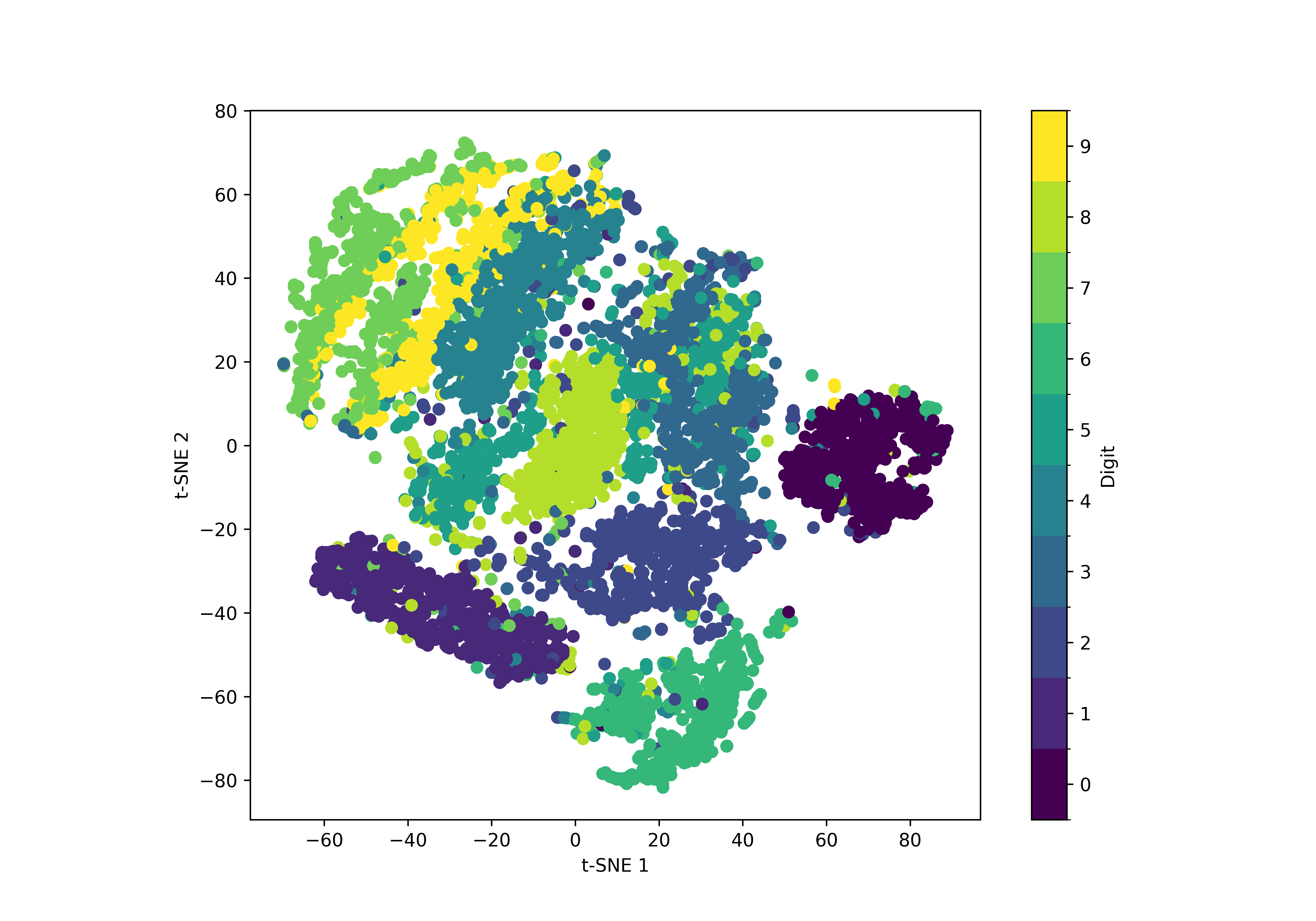
Fig. 23 The result of a t-SNE analysis of 7000 samples from the MNIST handwritten digits dataset.

Note

The result of this algorithm will likely give different results to the scikit-learn implementation. This is due to differences in how the optimisation of the KL divergence is performed.

t-SNE Algorithm

The t-SNE algorithm converts the distances between data points in the original space into probabilities. These probabilities represent the similarity between the data points. Then, in the lower dimensional description of the data, we aim to describe it by following the same probability distributions. This is achieved by minimising the Kullback-Leibler (KL) divergence between the low-dimensional data and original data probability distributions.

Let’s have a look at how that looks in Python code. We will apply this example to a simple example dataset with two overlapping clusters.

import pandas as pd

data = pd.read_csv('./../data/tsne-example.csv')

We can visualise this dataset with seaborn.

import matplotlib.pyplot as plt
import seaborn as sns

g = sns.PairGrid(data=data, hue='label')
g.map_upper(sns.scatterplot, s=15)
g.map_lower(sns.kdeplot)
g.map_diag(sns.kdeplot, lw=2)
plt.show()

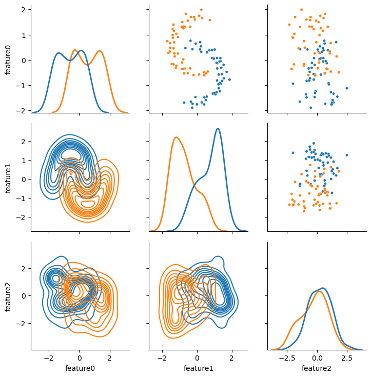
It is clear for this dataset that there are two “classes” of data. Indeed, the input file includes a label to help us see them visually. However, the spatial distribution of the two classes is a particular set that PCA is known to be poor at handling, look, in particular, at the cross plot between feature0 and feature1. Therefore, this is an interesting problem to see if t-SNE can improve over PCA.

Compute Similarities in Original Space

The first step in the t-SNE algorithm is to compute the similarities of the data points in the original space. This similarity is described by the probability that datapoint \(i\) would pick datapoint \(j\) as its neighbour in the original space. These probabilities are computed from a normal distribution centred around each point and normalised. Mathematically, this probability is computed as:

(34)\[ p_{j|i} = \frac{\exp{\left(\frac{-|x_i - x_j|^2}{2\sigma_i^2}\right)}}{\sum_{i\neq j}\exp{\left(\frac{-|x_i - x_j|^2}{2\sigma_i^2}\right)}}, \]

where \(|x_i - x_j|\) is the length of the vector between datapoints \(i\) and \(j\) and \(\sigma_i\) is determined for each observation \(i\) using a grid search based on the hyperparameter known as perplexity.

The first thing we will do to compute Eqn. (34) is finding a matrix of the vector magnitudes.

import numpy as np 

diff = data.values - data.values[:, np.newaxis]
norm = np.linalg.norm(diff, axis=-1)
np.fill_diagonal(norm, np.nan)

We set the diagonal of this matrix to be NaN as we are concerned with pairwise similarity, and the diagonal represents a datapoint’s similarity with itself. We compute \(\sigma_i\) from this matrix, which we achieve using a grid search across a range of values defined by the standard deviation in the vector length.

Note

Note that the np.nanstd function is used here to find the standard deviation, and the NaN values are ignored. We will continue to use nan* forms of NumPy functions throughout.

std_norm = np.nanstd(norm, axis=1)
sigma_search = np.linspace(0.01 * std_norm, 5 * std_norm, 200).T

We then calculate the probability, \(p_{j|i}(\sigma_i)\), for every value of \(\sigma_i\) in the grid search. Note that we ensure that the matrix of probabilities has no zeroes. Instead, these are replaced with the smallest positive floating point number your computer can describe; see the documentation for the `np. next after function.

p = np.exp(-(norm[:, :, np.newaxis] ** 2) / (2 * sigma_search ** 2))
epsilon = np.nextafter(0, 1)
p_norm = np.maximum(p / np.nansum(p, axis=0), epsilon)

/tmp/ipykernel_5589/1859251449.py:3: RuntimeWarning: invalid value encountered in divide
  p_norm = np.maximum(p / np.nansum(p, axis=0), epsilon)

The next step is then to compute the Shannon entropy for each value datapoint at each value of \(\sigma_i\) in the grid search,

\[ H[p_{j|i}(\sigma_i)] = - \sum_j p_{j|i}(\sigma_i) \log_2{[p_{j|i}(\sigma_i)]}. \]

H = -np.nansum(p_norm * np.log2(p_norm), axis=0)

To find the ideal value for \(\sigma_i\) for each data point, \(i\), we try to find the value of \(\sigma\) that results in a probability distribution with a perplexity that is as close as possible to the user-defined perplexity hyperparameter. The perplexity influences how the algorithm balances local and global structure in the data, with low perplexity leading to a focus on the closest individuals. Perplexity is conceptually related to the entropy of a probability distribution. It is defined as:

\[ \textrm{perplexity}(\sigma_i) = 2^{H[p_{j|i}(\sigma_i)]} \implies \frac{\textrm{perplexity}}{2^{H[p_{j|i}(\sigma_i)]}} = 1. \]

Therefore, if we take the logarithm of both sides,

\[ \ln[\textrm{perplexity}(\sigma_i)] - H[p_{j|i}(\sigma_i)] + \ln(2) = 0. \]

We will show this for a perplexity value of 9.

perplexity = 9

compare = np.abs(np.log(perplexity) - H + np.log(2))

The best \(\sigma_i\) for each datapoint is then the sigma_search values where compare is minimised.

sigma = sigma_search[range(sigma_search.shape[0]), compare.argmin(1)]

These sigma values are then used to calculate the similarities between the high dimensional data points.

p_ij = np.exp(-(norm ** 2) / (2 * sigma[:, np.newaxis] ** 2))
np.fill_diagonal(p_ij, 0)
p_ij = np.maximum(p_ij / np.nansum(p_ij, axis=1)[:, np.newaxis], epsilon)

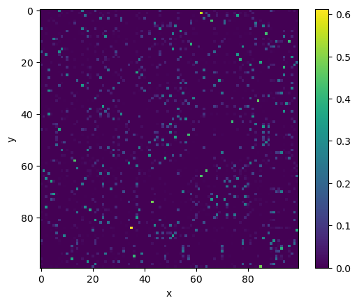
We can visualise this probability matrix with the imshow function from matplotlib:

fig, ax = plt.subplots()

_ = ax.imshow(p_ij)
ax.set_xlabel('x')
ax.set_ylabel('y')
fig.colorbar(_)
plt.show()

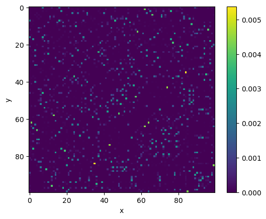
One thing you may note is that this matrix is not symmetrical. We currently are computing the conditional probabilities, \(p_{j|i}\), not the joint probability, \(p_{ij}\). We can convert to the joint probabilities with the following,

\[ p_{ij} = \frac{p_{j|i} + p_{i|j}}{2n}, \]

where \(n\) is the number of data points.

p_ij_symmetric = (p_ij + p_ij.T) / (2 * p_ij.shape[0])
p_ij_symmetric = np.maximum(p_ij_symmetric, epsilon)

fig, ax = plt.subplots()

_ = ax.imshow(p_ij_symmetric)
ax.set_xlabel('x')
ax.set_ylabel('y')
fig.colorbar(_)
plt.show()

Creating Initial Guesses for Lower Dimensionality Datapoints

Now that we have the affinities of the high dimensional data, we can create some initial guesses for the lower dimensional data. We want to end up with data in two dimensions. One of the most popular ways to produce this initial guess is to use singular value decomposition.

n_dimensions = 2

U, S, Vt = np.linalg.svd(data)
pca = data @ Vt.T[:, :n_dimensions]
pca.columns = ['PC1', 'PC2']
pca['label'] = data['label']

sns.jointplot(data=pca, x='PC1', y='PC2', hue='label', kind='scatter')
plt.show()

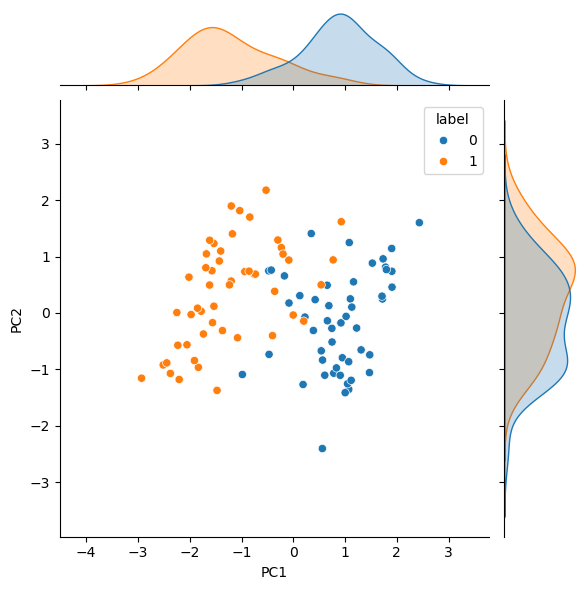
Unsurprisingly, the SVD, i.e., a PCA approach, is ineffective in disambiguating the data. Let’s see if t-SNE can improve on this by using the PCA results as the starting configuration.

Minimising the Kullback-Leibler (KL) Divergence

As mentioned above, t-SNE minimises the KL divergence of affinities between the different spaces. Therefore, we need to be able to compute the affinity of the lower dimensional space (we will use \(y\) for the lower dimension data). This is achieved by considering a Student’s t-distribution (hence the t in t-SNE) with one degree of freedom,

\[ q_{ij} = \frac{(1 + |y_i - y_j| ^ 2) ^{-1}}{\sum_{i\neq l}(1 + | y_i - y_l | ^ 2) ^{-1}}. \]

Since this is something that will change to minimise the KL divergence, as new lower-dimensional positions are generated, we will put this in a function.

def low_dimensional_affinity(y):
    """
    Calculates the low dimensional affinity matrix for t-SNE.
    
    :param y: (np.ndarray) should be a flattened array of the low dimensional data. 
    
    :returns qq_ij: (np.ndarray) the low dimensional affinity matrix.
    """
    y = y.reshape(-1, n_dimensions)
    diff = y - y[:, np.newaxis]
    norm = np.linalg.norm(diff, axis=-1)

    qq_ij = (1 + norm ** 2) ** (-1)
    np.fill_diagonal(qq_ij, 0)
    qq_ij = qq_ij / qq_ij.sum()

    epsilon = np.nextafter(0, 1)
    qq_ij = np.maximum(qq_ij, epsilon)
    return qq_ij

The function we are then looking to minimise, using scipy.optimize.minimize, is then as follows:

from scipy.optimize import minimize
from scipy.special import kl_div

def to_minimise(y):
    qq_ij = low_dimensional_affinity(y)
    return kl_div(p_ij_symmetric, qq_ij).sum()

We return the results of the minimisation to the res object. Similar to the PCA results above, this can be plotted with a histogram to see how the t-SNE algorithm has transformed the data.

res = minimize(to_minimise, pca.values[:, :2].flatten())
tsne_transformed = res.x.reshape(-1, 2)
data['tSNE1'] = tsne_transformed[:, 0]
data['tSNE2'] = tsne_transformed[:, 1]

sns.jointplot(data=data, x='tSNE1', y='tSNE2', hue='label', kind='scatter')
plt.show()

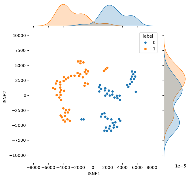
For this non-linearly discriminated data, the t-SNE algorithm is much better at finding a reduced dimensionality that allows the differences to be investigated. Let us continue to look at t-SNE, as it is available from scikit-learn.