Kernel Tricks#
So far, our support vector machines are only realistically able to classify data where there is a linear trend. While this is often the case – in particular in high dimensional spaces of neural networks – it is valuable to use these tools on non-linear systems. The approach in SVMs is to harness the kernel trick, akin to something we have seen in linear algebra.
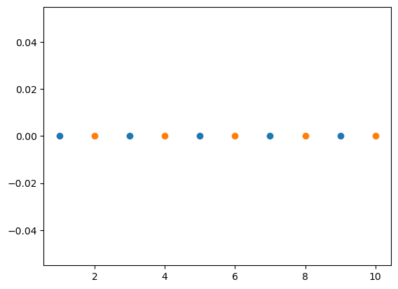
This trick transforms the space that the data are in. Usually, this transformation involves taking data to a high-dimensional space, creating a linear discrimination in the data. A popular example of a kernel trick is for one-dimensional data, where each data point is an integer. Consider the classification of odd and even numbers.
import numpy as np

odd = np.arange(1, 11, 2)
even = np.arange(2, 11, 2)
This is impossible in the current mapping.
import matplotlib.pyplot as plt

fig, ax = plt.subplots()

ax.plot(odd, np.zeros_like(odd), 'o')
ax.plot(even, np.zeros_like(even), 'o')
plt.show()
However, by computing the modulus of x, we can see a linear discrimination between the classes.
fig, ax = plt.subplots()

ax.plot(odd, np.mod(odd, 2), 'o')
ax.plot(even, np.mod(even, 2), 'o')
plt.show()
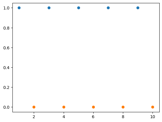
Notice that a support vector machine hyperplane above would sit along \(y = 0.5\).
Naturally, this is a simplistic approach.
The radial basis function kernel is one of the most popular kernels and is the default for the scikit-learn implementation of support vector machines.
This kernel is based on a Gaussian distribution and remaps data to a higher dimensionality space.
In some ways, this can be thought of as the inverse of the dimensionality reduction approach of t-SNE.
We will see the kernel trick in action later.