Integration

Integration is often introduced as the inverse of differentiation. Indeed, to calculate the integral of some function, we just performed the opposite operation to Eqn. (31). However, when discussing integration in a graphical context, we are told that the integral is the area under a curve drawn by the function. Here, I want to show how these two facts are analogous.

Rectangle Method

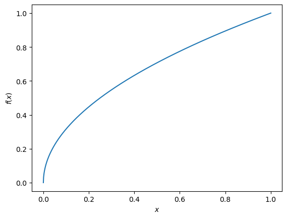
Let’s consider some function \(f(x) = \sqrt{x}\). We can plot this with matplotlib.

import numpy as np
import matplotlib.pyplot as plt

x = np.linspace(0, 1, 1000)
y = np.sqrt(x)

fig, ax = plt.subplots()

ax.plot(x, y)
ax.set_xlabel('$x$')
ax.set_ylabel('$f(x)$')
plt.show()

If we want to estimate the area under this curve, from \(x=0.2\) to \(x=0.8\), we can imagine drawing a rectangle with a width of 0.6 and height of \(f(0.2)\).

fig, ax = plt.subplots()

x_area = [0.2]
y_area = np.sqrt([0.2])

ax.plot(x, y)
ax.bar(x_area, y_area, align='edge', 
       width=np.diff([0.2, 0.8]), alpha=0.5)
ax.set_xlabel('$x$')
ax.set_ylabel('$f(x)$')
plt.show()

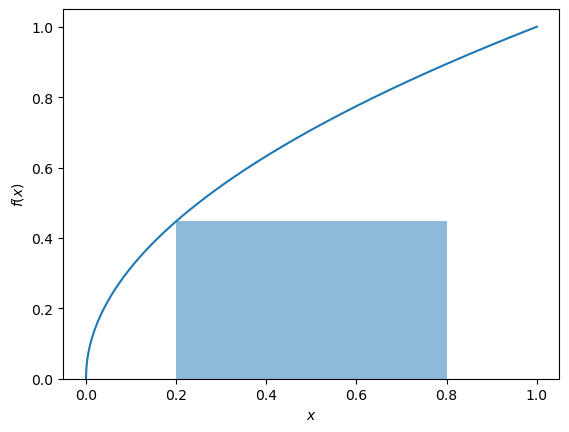
The area of this rectangle is as follows:

np.diff(x_area) * np.sqrt(0.2)

array([], dtype=float64)

This is a poor estimate of the area under the curve. The only part where the rectangle meets the curve is at \(x=0.2\). However, what if we had a few rectangles and added up the individual areas? We can use rectangles with a \(\text{d}x\) width.

Note

The slightly strange np.linspace arguments are necessary to overcome floating-point round-off errors.

fig, ax = plt.subplots()

dx = 0.1
x_area = np.arange(2, 8, dx * 10) / 10
y_area = np.sqrt(x_area)

ax.plot(x, y)
ax.bar(x_area, y_area, align='edge', 
       width=np.diff(x_area)[0], alpha=0.5)
ax.set_xlabel('$x$')
ax.set_ylabel('$f(x)$')
plt.show()

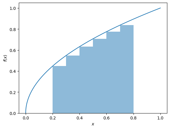
This is a slightly better estimate of the area under the curve.

np.sum(dx * y_area)

0.3945755162000907

If we continue this process, taking narrower and narrower rectangles, we should eventually reach a reasonable estimate of the area. This can be said mathematically as \(\text{d}x \to 0\), the sum of the rectangles tends towards the true area.

fig, ax = plt.subplots()

dx = 0.0001
x_area = np.arange(0.2, 0.8, dx)
y_area = np.sqrt(x_area)

ax.plot(x, y)
ax.bar(x_area, y_area, align='edge', 
       width=dx, alpha=0.5)
ax.set_xlabel('$x$')
ax.set_ylabel('$f(x)$')
plt.show()

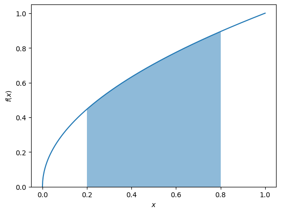
Which are can be calculated as follows.

np.sum(dx * y_area)

0.41746643737342515

This is known as the rectangle method for computing integrals; it is a type of Riemann sum. It is commonly used in computation to find the value of an integral numerically. We note here that other approaches to compute integrals numerically exist, i.e., the trapezoidal rule.

Why Is the Integral the Opposite of a Derivative?

For some finite \(\text{d}x\), the estimate of the integral of \(f(x)\) from \(x=0.2\) to \(x=0.8\), which we will call \(g\), can be written with the following sum,

\[ g = \sum_{x=0.2}^{0.8} f(x) \;a\text{d}x. \]

When \(\text{d}x\) is infinitesimally small, we use the following integral notation,

\[ g = \int_{0.2}^{0.8} fx \;\text{d}x. \]

We can replace \(0.8\) with the variable \(x_2\), so the function \(g\) now depends on \(x_2\).

\[ g(x_2) = \int_{0.2}^{x_2} fx \;\text{d}x. \]

The difference in the integral where \(x_2=0.8\) and \(x_2=0.9\) is shown below.

x_area2 = np.arange(0.8, 0.9, dx)
y_area2 = np.sqrt(x_area2)

fig, ax = plt.subplots()

ax.plot(x, y)
ax.bar(x_area, y_area, align='edge', 
       width=dx, alpha=0.5)
ax.bar(x_area2, y_area2, align='edge', 
       width=dx, alpha=0.5)
ax.set_xlabel('$x$')
ax.set_ylabel('$f(x)$')
plt.show()

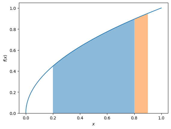
The value of this change in area can be written as

\[ \text{d}g(x_2) = f(x_2)\;\text{d}x, \]

which can be rearranged to give,

\[ \frac{\text{d}g(x_2)}{\text{d}x} = f(x_2). \]

This tells us that the derivative of any function that gives the area of a graph is equal to the function itself, showing the anti-derivative nature of integrals.

What About the Offset?

If we consider curves, \(y_1 = x^2\) and \(y_2 = x^2 + 1\), you may notice that these have the same derivative, but the area under the curve would be different (by values of \(1\)).

x = np.linspace(-1, 1, 1000)
y1 = x ** 2
y2 = x ** 2 + 1

fig, ax = plt.subplots()

ax.plot(x, y1)
ax.plot(x, y2)
ax.set_xlabel('$x$')
ax.set_ylabel('$y$')
plt.show()

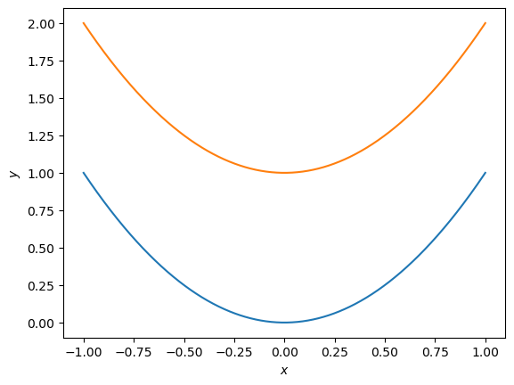
This is where the constant \(C\) arises from the condition of an indefinite integral. This is to say, one where there are no bounds (the subscript and superscript values around the integral).

Integrals in Python

We have already seen how an integral may be computed numerically in Python using some Riemann sum. But, similar to differentiation, we can use the sympy library to compute integrals symbolically.

from sympy import symbols, integrate

x = symbols('x')

integrate(x ** 0.5, x)

\[\displaystyle 0.666666666666667 x^{1.5}\]

This matches with the result from the general formula, the inverse of Eqn. (31),

\[ \int x^n \text{d}x = \frac{x^{n+1}}{n+1} + C, \]

where \(n \neq -1\). We can use this to check the result of our summation above by computing the difference between the results of the above equation at \(x=0.8\) and \(x=0.2\).

Note

The subs method will substitute a numerical value for a given symbol.

integrate(x ** 0.5, x).subs(x, 0.8) - integrate(x ** 0.5, x).subs(x, 0.2)

\[\displaystyle 0.417399355799961\]

This matches well the result from the rectangle method with a small \(\text{d}x\).