Linear Transformations

A linear transformation is a way to map between two different vector spaces. Previously, basis vectors were introduced as the vectors that define some vector space. Consider just a single vector, \(\mathrm{r}\), in the vector space that was introduced in Fig. 6.

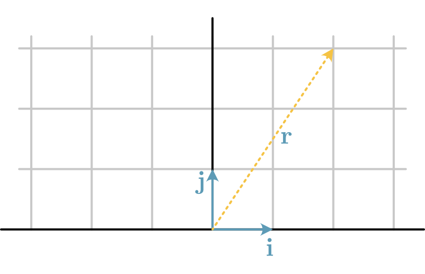
Fig. 11 The basis vectors \(\mathbf{i}\) and \(\mathbf{j}\) defining the coordinate system for a single vector.

The basis vector \(\mathbf{i}\) is a vector that goes one step right along the x-axis and zero steps up along the y-axis. Meanwhile, the \(\mathbf{j}\) basis vector goes zero steps along the x-axis and one up the yaxis. These initial basis vectors can be written as,

(9)\[\begin{split} \mathbf{i} = \begin{bmatrix} 1 \\ 0 \end{bmatrix}, \;\;\;\;\;\;\mathbf{j} = \begin{bmatrix} 0 \\ 1 \end{bmatrix}. \end{split}\]

These are not the only basis vectors that can be used to describe a vector space. Consider the rotation of the basis vectors (and associated vector) shown in Fig. 12, where the vectors have been rotated 90° anti-clockwise around the origin.

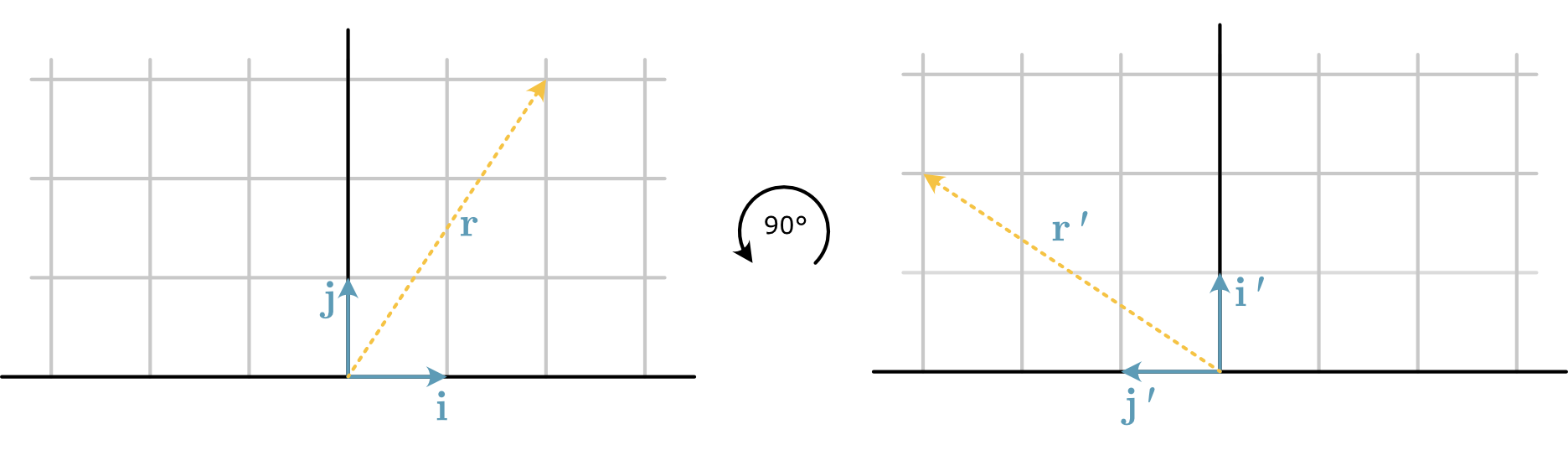
Fig. 12 The 90° rotation from the initial basis set of vectors to the new set, \(\mathbf{i'}\) and \(\mathbf{j'}\) and the corresponding rotation of the vector \(\mathbf{r}\).

This rotation is a linear transformation, which results in a new basis set of vectors. These new vectors are the same length as the initial set, but now \(\mathbf{i'}\) is going straight up by a single step and \(\mathbf{j'}\) going back one step along the x-axis.

It is possible to write this new basis set of vectors in terms of the initial basis set,

(10)\[ \mathbf{i'} = 0\mathbf{i} + 1\mathbf{j}, \;\;\;\;\;\;\; \mathbf{j'} = -1\mathbf{i} + 0\mathbf{j}. \]

The new position of the vector \(\mathbf{r}\) following the change of basis set is \((2\mathbf{i'} + 3\mathbf{j'})\). Then by using substitution from Eqn. (10) it is possible to find the new position of \(\mathbf{r}\) in the initial basis set,

(11)\[\begin{split} \begin{aligned} \mathbf{r'} & = 2\mathbf{i'} + 3\mathbf{j'} \\ & = 2(0\mathbf{i} + 1\mathbf{j}) + 3(-1\mathbf{i} + 0\mathbf{j}) \\ & = 0\mathbf{i} + 2\mathbf{j} - 3\mathbf{i} + 0\mathbf{j} \\ & = -3\mathbf{i} + 2 \mathbf{j}. \end{aligned} \end{split}\]

Here, the basis set of vectors is been used to transform from one vector space to another. The result of this transformation is the rotation of the vector \(\mathbf{r}\) 90° anti-clockwise around the origin.

Inverse Linear Transformations

Of course, for every linear transformation, there exists an inverse, which performs the opposite mapping. So for the anti-clockwise rotation shown in Fig. 12 there is an inverse that rotates 90° clockwise. The basis set of vectors for this linear transformation would be

(12)\[ \mathbf{i'} = 0\mathbf{i} - 1\mathbf{j}, \;\;\;\;\;\;\; \mathbf{j'} = 1\mathbf{i} + 0\mathbf{j}. \]

The ability to describe linear transformations with matrices which will be discussed later, will help with the definition of inverse linear transformations. Performing linear transformations of vectors is extremely important in a range of applications across scientific computing, from the modelling of molecules in chemistry to the development of computer graphics that appear in video games.