Comparing Classification Methods#
Let’s now compare the different classification methods we have discussed.
Instead of using our own implementations, we will harness the more efficient implementations of scikit-learn.
We will test each of them with the breast cancer dataset, so we can start by loading this dataset.
import pandas as pd

data = pd.read_csv('./../data/breast-cancer.csv')
data
| Diagnosis | Radius | Texture | Perimeter | Area | Smoothness | Compactness | Concavity | Concave Points | Symmetry | Fractal Dimension | |
|---|---|---|---|---|---|---|---|---|---|---|---|
| 0 | Malignant | 17.99 | 10.38 | 122.80 | 1001.0 | 0.11840 | 0.27760 | 0.30010 | 0.14710 | 0.2419 | 0.07871 |
| 1 | Malignant | 20.57 | 17.77 | 132.90 | 1326.0 | 0.08474 | 0.07864 | 0.08690 | 0.07017 | 0.1812 | 0.05667 |
| 2 | Malignant | 19.69 | 21.25 | 130.00 | 1203.0 | 0.10960 | 0.15990 | 0.19740 | 0.12790 | 0.2069 | 0.05999 |
| 3 | Malignant | 11.42 | 20.38 | 77.58 | 386.1 | 0.14250 | 0.28390 | 0.24140 | 0.10520 | 0.2597 | 0.09744 |
| 4 | Malignant | 20.29 | 14.34 | 135.10 | 1297.0 | 0.10030 | 0.13280 | 0.19800 | 0.10430 | 0.1809 | 0.05883 |
| ... | ... | ... | ... | ... | ... | ... | ... | ... | ... | ... | ... |
| 564 | Malignant | 21.56 | 22.39 | 142.00 | 1479.0 | 0.11100 | 0.11590 | 0.24390 | 0.13890 | 0.1726 | 0.05623 |
| 565 | Malignant | 20.13 | 28.25 | 131.20 | 1261.0 | 0.09780 | 0.10340 | 0.14400 | 0.09791 | 0.1752 | 0.05533 |
| 566 | Malignant | 16.60 | 28.08 | 108.30 | 858.1 | 0.08455 | 0.10230 | 0.09251 | 0.05302 | 0.1590 | 0.05648 |
| 567 | Malignant | 20.60 | 29.33 | 140.10 | 1265.0 | 0.11780 | 0.27700 | 0.35140 | 0.15200 | 0.2397 | 0.07016 |
| 568 | Benign | 7.76 | 24.54 | 47.92 | 181.0 | 0.05263 | 0.04362 | 0.00000 | 0.00000 | 0.1587 | 0.05884 |
569 rows × 11 columns
This is a labelled dataset where the labels are either Malignant or Benign. To use these in many of our algorithms, we need to encode these to numerical values.
data['Encoded Diagnosis'] = data['Diagnosis'].apply(lambda x: 1 if x == 'Malignant' else 0)
Let’s split the data into our usual training and test subsets.
from sklearn.model_selection import train_test_split

train, test = train_test_split(data, test_size=0.2, random_state=42)
We will then scale the data. This is not necessarily required for all of the algorithms, but for consistency, we will use it in all cases.
from sklearn.preprocessing import StandardScaler

scaler = StandardScaler()
scaled_train = scaler.fit_transform(train.drop(['Diagnosis', 'Encoded Diagnosis'], axis=1))
scaled_test = scaler.fit_transform(test.drop(['Diagnosis', 'Encoded Diagnosis'], axis=1))
Since all methods have a shared API, we can use a loop to perform each method in turn. For each method, we train using the training share and then make predictions on the test data.
from sklearn.linear_model import LogisticRegression
from sklearn.svm import SVC
from sklearn.ensemble import RandomForestClassifier

methods = {'Logistic Regression': LogisticRegression(random_state=42),
           'SVM': SVC(random_state=42),
           'Random Forest': RandomForestClassifier(random_state=42)}

for k, v in methods.items():
    v.fit(scaled_train, train['Encoded Diagnosis'])
    test[f'{k} Prediction'] = v.predict(scaled_test)
Metrics#
To quantify the success of a machine learning workflow, numerical quality scores are necessary.
So far, we have used accuracy_score; however, this is not an ideal metric as it only accounts for when the algorithm has identified true positives.
Other popular metrics include precision, recall, and the combinations of these two, the F1-score.
Precision tells us how the many of the samples that are identified as malignant were, in fact, malignant,
The recall answers how many of the malignant samples were correctly identified by the algorithm,
Finally, the F1-score balances these two and is a valuable tool when a single metric is needed.
The true and false positives and negatives are described in Fig. 30.
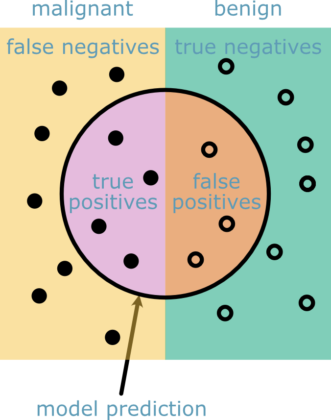
Fig. 30 A figure showing the identification of true and false positives and negatives that make up the precision and recall scores.#
These metrics are computed with sklearn, as shown below.
from sklearn.metrics import precision_score, recall_score, f1_score

for k in methods.keys():
    print(f'{k} Precision: {precision_score(test["Encoded Diagnosis"], test[f"{k} Prediction"]):.3f}')
    print(f'{k} Recall: {recall_score(test["Encoded Diagnosis"], test[f"{k} Prediction"]):.3f}')
    print(f'{k} F1-Score: {f1_score(test["Encoded Diagnosis"], test[f"{k} Prediction"]):.3f}')
    print()
Logistic Regression Precision: 1.000
Logistic Regression Recall: 0.907
Logistic Regression F1-Score: 0.951

SVM Precision: 1.000
SVM Recall: 0.930
SVM F1-Score: 0.964

Random Forest Precision: 0.975
Random Forest Recall: 0.907
Random Forest F1-Score: 0.940
All three methods do very well in the classification. Indeed, the scikit-learn implementation outperform the implementations we wrote ourselves. However, from comparing the F1-scores, the support vector machine is the most effective. We highlight here that the implementations used are naïve, in that there is no hyperparameter optimisation being used. To achieve this, one could consider performing some random search or optimisation over the hyperparameter space.