Priors

In the previous page, we introduced Bayes’ theorem, which inverts conditional probabilities. The form of Bayes’ theorem we met was,

\[ p(A | B) = \frac{p(B | A) p(A)}{p(B)}. \]

Note

It is slightly unfair to call these prior uninformative, given they inform on the minimum and maximum values that can be taken. However, this name is popular in the field.

In this form, \(p(A)\) is the prior probability or simply the prior. It ensures that what we already know about the world is included in our analysis. We achieve this, for example, by saying that our parameter \(A\) cannot be less than 0 and cannot be greater than 1. This way, we would use a uniform prior probability distribution. We imposed this uninformative prior when implementing PyMC using the pm.Uniform objects for our parameters.

Informative Priors

One of the important benefits of the Bayesian approach is to take advantage of what we already know about the world. We will come back to highlight this impact in the next section. Consider how we can create a meaningful prior probability based on some prior measurement.

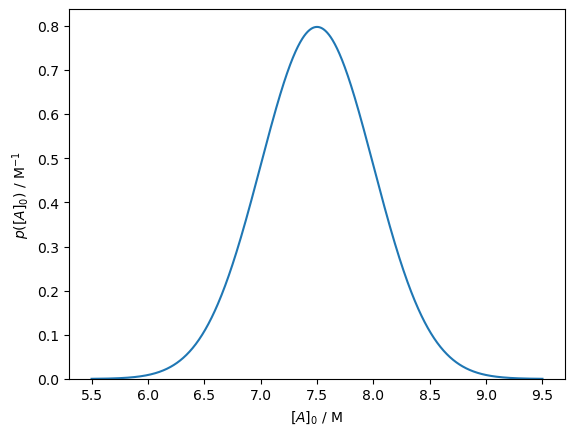
Consider if we are trying to determine the rate constant, \(k\), and the concentration of \(A\) at time \(0\) in the previous example. When we prepare the experiment, we have some understanding of the initial concentration, for example, from the preparation of our system. Therefore, we can say that the initial concentration is 7.5 ± 0.5 M. This can be described with a normal probability distribution, which we visualise below.

import numpy as np
import matplotlib.pyplot as plt 
from scipy.stats import norm

mu = 7.5 
sigma = 0.5 

A_0 = norm(mu, sigma)
x = np.linspace(mu - 4 * sigma, mu + 4 * sigma, 1000)

fig, ax = plt.subplots()
ax.plot(x, A_0.pdf(x))
ax.set_xlabel('$[A]_0$ / M')
ax.set_ylabel('$p([A]_0)$ / M$^{-1}$')
ax.set_ylim(0, None)
plt.show()

We may also consider where there are some complementary measurements; for example, some previous work may have measured the rate constant, \(k\), that we are interested in. Consider if the previous work measured \(k\) as 0.15 ± 0.01 s^-1, which we can present as shown.

mu = 0.15
sigma = 0.01 

k = norm(mu, sigma)
x = np.linspace(mu - 4 * sigma, mu + 4 * sigma, 1000)

fig, ax = plt.subplots()
ax.plot(x, k.pdf(x))
ax.set_xlabel('$[A]_0$ / M')
ax.set_ylabel('$p([A]_0)$ / M$^{-1}$')
ax.set_ylim(0, None)
plt.show()

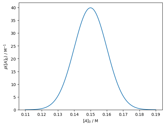
You may notice that this prior probability is very low at the maximum likelihood estimation of \(k\).

k.pdf(0.1046)

0.0013340066490355885

Therefore, this prior knowledge may be influential in the estimation of the probability of the model, given the data. This is an important input in our analysis so that we can look at this calculation now.

The Subjectivity of Priors

Opponents of Bayesian modelling claim that using a prior is a bias to get the answer you want. This is a fair argument, so to counter it, Bayesian practitioners must be explicit about why they picked particular priors and justify their decisions. For example, if you chose some normally distributed prior around some value, it is important that you state why this was selected.