Using PyMC

Using PyMC#

PyMC is a very powerful Python library designed for probabilistic and Bayesian analysis. Here, we show that PyMC can be used to perform the same likelihood sampling that we previously wrote our own algorithm for.

Below, we read in the data and build the model.

import pandas as pd 
import numpy as np
from scipy.stats import norm

data = pd.read_csv('../data/first-order.csv')

D = [norm(data['At'][i], data['At_err'][i]) for i in range(len(data))]

def first_order(t, k, A0):
    """
    A first order rate equation.
    
    :param t: The time to evaluate the rate equation at.
    :param k: The rate constant.
    :param A0: The initial concentration of A.
    
    :return: The concentration of A at time t.
    """
    return A0 * np.exp(-k * t)

The next step is to construct the PyMC sampler. The format that PyMC expects can be a bit unfamiliar.

First we create objects for the two parameters, these are bounded so \(0 \leq k < 1\) and \(0 \leq [A]_0 < 10\). Strictly, these are prior probabilities, which we will look at next, but using uniform distributions means this is mathematically equivalent to likelihood sampling. Next, we create a normally distributed likelihood function to compare the data and the model. Finally, we sample for 1000 steps, with 10 chains. The tune parameter is the number of steps for tuning the Markov chain step sizes.

import pymc as pm

with pm.Model() as model:
    k = pm.Uniform('k', 0, 1)
    A0 = pm.Uniform('A0', 0, 10)
    
    At = pm.Normal('At', 
                   mu=first_order(data['t'], k, A0), 
                   sigma=data['At_err'], 
                   observed=data['At'])
    
    trace = pm.sample(1000, tune=1000, chains=10, progressbar=False)

Initializing NUTS using jitter+adapt_diag...

Multiprocess sampling (10 chains in 2 jobs)

NUTS: [k, A0]

Sampling 10 chains for 1_000 tune and 1_000 draw iterations (10_000 + 10_000 draws total) took 4 seconds.

Unlike the code that we created previously, PyMC defaults to using the NUTS sampler, which stands for No-U-Turn sampler [7]. This sampler enables the step size tuning that we have taken advantage of.

This results in a object assigned to the variable trace.

trace

arviz.InferenceData

posterior
sample_stats
observed_data

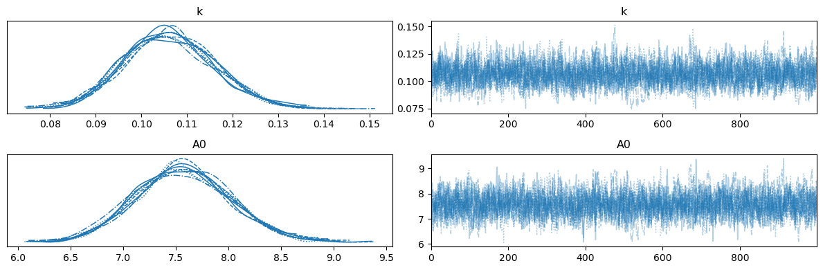
This contains the chain information amoung other things. Instead of probing into the trace object, we can take advantage of functionality from the arviz library to produce some informative plots.

import matplotlib.pyplot as plt
import arviz as az

az.plot_trace(trace, var_names=["k", "A0"])
plt.tight_layout()
plt.show()

../_images/65cb9ef6040296236f07836d24c55f074494a7214afb25596285e4ad74e9d1b7.png

Above, we can see the trace of each of the different chains. The chains appear to have converged to the same distribution. We can get the flat chains with the following function.

flat_chain = np.vstack([trace.posterior['k'].values.flatten(), trace.posterior['A0'].values.flatten()]).T

import seaborn as sns

chains_df = pd.DataFrame(flat_chain, columns=['k', 'A0'])
sns.jointplot(data=chains_df, x='k', y='A0', kind='kde')
plt.show()

../_images/e8b2e20723372e14f816dc41ba27d1fedce1a83f2867fc40cf801b8bbb085704.png

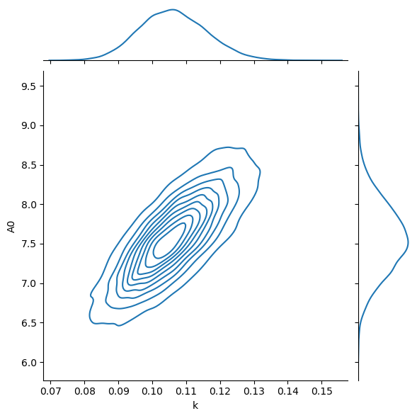
It is clear that, using PyMC, we have much better sampling of the distributions. This makes using summary statistics, like the mean and standard deviation much more reliable.

az.summary(trace, var_names=["k", "A0"])

	mean	sd	hdi_3%	hdi_97%	mcse_mean	mcse_sd	ess_bulk	ess_tail	r_hat
k	0.106	0.01	0.088	0.125	0.000	0.000	2799.0	3562.0	1.0
A0	7.572	0.45	6.716	8.397	0.009	0.006	2729.0	3228.0	1.0