Multilayer Perceptron

It was highlighted previously that the perceptron (the base unit for the artificial neural networks), capable of some simple logic, cannot implement an exclusive OR operation. This led to a significant decrease in excitement about artificial intelligence. However, the XOR operation can be performed with the inclusion of just a single hidden layer. We can see a diagram of this simple artificial neural network in Fig. Fig. 37.

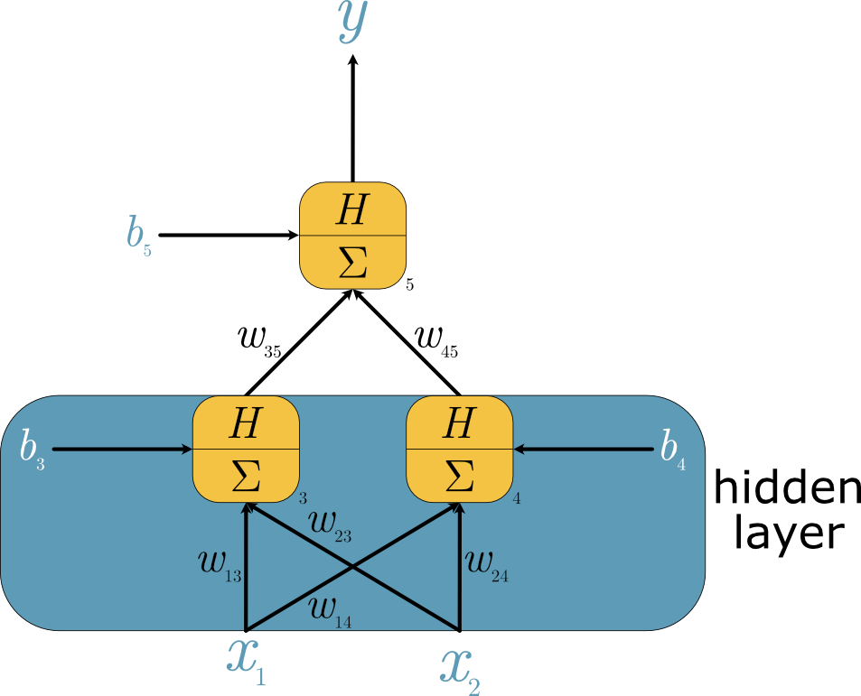
Fig. 37 A pictorial description of a multilayer perceptron, where the activation function, \(H\), is the Heaviside function and the transfer function is a summation, \(\Sigma\), for all nodes.

In Fig. Fig. 37, the hidden layer is fully connected, meaning all the nodes are connected to all the inputs. This is probably the most straightforward artificial neural network, so let’s write some simple Python code to implement it. We will start with defining the Heaviside function again.

import numpy as np

def heaviside(x):
    """
    Heaviside step function.
    
    :param x: input value
    
    :return: 1 if x >= 0, 0 otherwise
    """
    return np.where(x < 0, 0, 1)

The network above takes two inputs, \(\mathbf{x} = \begin{bmatrix} x_1 \\ x_2 \end{bmatrix}\), which we will define below.

x = np.array([[0, 0],
              [0, 1],
              [1, 0],
              [1, 1]])
x

array([[0, 0],
       [0, 1],
       [1, 0],
       [1, 1]])

Now, we will define the weights and bias between our input and hidden layer. For the weights, we will define this as a 2×2 matrix. Here, we will define these with random values.

rng = np.random.RandomState(42)
layer_one_weights = rng.randn(2, 2)
layer_one_biases = rng.randn(2) 
layer_one_weights, layer_one_biases

(array([[ 0.49671415, -0.1382643 ],
        [ 0.64768854,  1.52302986]]),
 array([-0.23415337, -0.23413696]))

The transfer function is a summation so that we can perform the matrix multiplication of the inputs and the weights with a dot product. And, again, the activation function is a Heaviside function.

layer_one_outputs = heaviside(np.dot(x, layer_one_weights) + layer_one_biases)
layer_one_outputs

array([[0, 0],
       [1, 1],
       [1, 0],
       [1, 1]])

These outputs are then fed from the hidden layer to the output layer. There are only two weights and one bias this time, but we will initialise these randomly again.

layer_two_weights = rng.randn(2, 1)
layer_two_biases = rng.randn(1)
output = heaviside(np.dot(layer_one_outputs, layer_two_weights) + layer_two_biases)
output

array([[0],
       [1],
       [1],
       [1]])

The first, second, and third results match the trust table. However, the final does not. Therefore, we must optimise the weights and biases. In machine learning parlance, we would call this training, but the logic is similar to optimisation, even if the approaches are not always the same.

Let’s look at how artificial neural networks are trained.