Likelihood

Note

Note the capital \(\Theta\) to indicate a vector of parameters.

An important concept in probabilistic modelling is the likelihood, often written as \(p[D | M(\Theta)]\). We read this as the probability that some data, \(D\), would be observed given an underlying model, \(M\), with parameters \(\Theta\), which generates the data. Naturally, the higher this probability, the more likely that \(D\) would be observed. Let’s think about this for a straightforward model and data.

Simple Example

We will start with a single data point, which is a normal distribution with a mean of 2.52 and a standard deviation of 0.65. Let’s create a scipy.stats object to describe this, called D (for data).

from scipy.stats import norm

D = norm(2.52, 0.62)

Now we need a model, \(M\), with one parameter, \(\theta\),

\[ M(\theta) = \theta ^ 2. \]

We can write a simple function to describe this,

def M(theta):
    """
    Our model function.
    
    :param theta: The parameter to evaluate the model at.
    :return: The value of the model at theta.
    """
    return theta ** 2

We can compute the likelihood of a given \(\theta\) as the probability density function of the data at \(M(\theta)\). So for \(\theta\) of 1.5, we find the following.

D.pdf(M(1.5))

0.5852443461687209

So the probability that the data, \(D\), would be observed given the model, \(M(1.5)\), \(p[D | M(1.5)] \approx 0.59\). We can present this visually with a plot.

import numpy as np
import matplotlib.pyplot as plt

data_range = np.linspace(0, 5, 1000)

fig, ax = plt.subplots()

ax.fill_between(data_range, D.pdf(data_range))
ax.plot(M(1.5), D.pdf(M(1.5)), 'ko')
ax.set_xlabel(r'$M(\theta$)')
ax.set_ylabel(r'$p[D|M(\theta)]$')
ax.set_ylim(0, None)
plt.show()

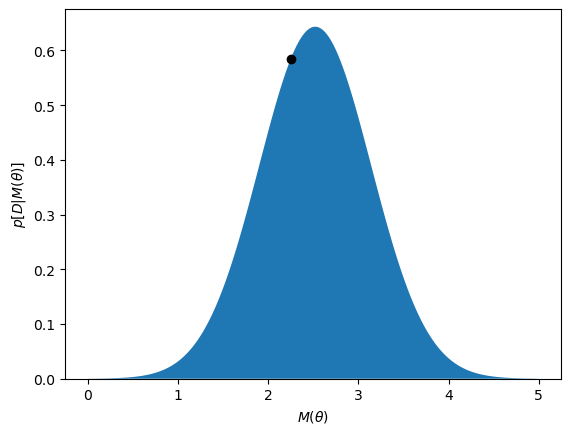
We can see that the black dot, which indicates \(M(1.5)\), is not at the top of the probability density function. We say that the likelihood is not maximised. A simple optimisation algorithm can be used to maximise the likelihood.

Note

Recall that the minimum is the same as the negative maximum.

from scipy.optimize import minimize

def negative_likelihood(theta):
    """
    The negative likelihood function.
    
    :param theta: The parameter to evaluate the negative likelihood at.
    :return: The negative likelihood at theta.
    """
    return -D.pdf(M(theta))

res = minimize(negative_likelihood, 1.5)
res.x

array([1.58745045])

We can see that the likelihood is maximised at a value of \(\theta\) of around 1.59.

fig, ax = plt.subplots()

ax.fill_between(data_range, D.pdf(data_range))
ax.plot(M(res.x), D.pdf(M(res.x)), 'ko')
ax.set_xlabel(r'$M(\theta$)')
ax.set_ylabel(r'$p[D|M(\theta)]$')
ax.set_ylim(0, None)
plt.show()

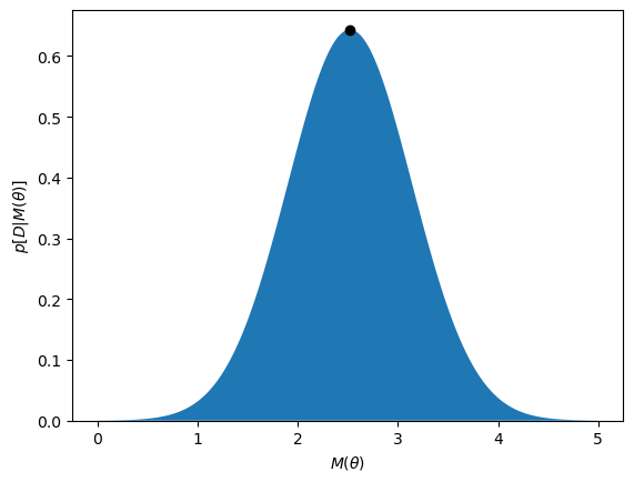
This looks like the maximum has been found, now we can extend it to a more complex data set.

Fitting a Model to Data

Let’s bring back the data from the previous section.

import pandas as pd 

data = pd.read_csv('../data/first-order.csv')

fig, ax = plt.subplots()
ax.errorbar(data['t'], data['At'], data['At_err'], fmt='o')
ax.set_xlabel('Time / s')
ax.set_ylabel('[A] / M')
plt.show()

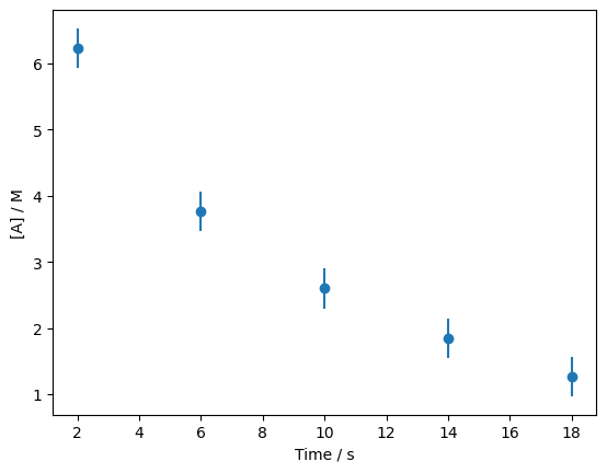
As was mentioned, this data describes the concentration of a chemical species, \([A]\), as a function of time, \(t\) during some reaction. This is known to follow what is called a first-order rate law, which has the following form,

(38)\[ [A]_t = [A]_0\exp{(-kt)}, \]

where \([A]_t\) is the concentration at time \(t\), \([A]_0\) is the starting concentration, and \(k\) is the rate constant, which describes the speed of the reaction. We can write the following function that describes this model.

def first_order(t, k, A0):
    """
    A first order rate equation.
    
    :param t: The time to evaluate the rate equation at.
    :param k: The rate constant.
    :param A0: The initial concentration of A.
    
    :return: The concentration of A at time t.
    """
    return A0 * np.exp(-k * t)

This equation is our model, \(M(\Theta)\), with parameters \(\Theta = [k,\;[A]_0]\).

To compute the likelihood of the data given some values of \(\Theta\) requires the data can be describes as a statistical distribution. We can achieve this by describing each datapoint with a normal distribution.

D = [norm(data['At'][i], data['At_err'][i]) for i in range(len(data))]

The Multivariate Normal Distribution

Note, that this same process could be achieved using a multivariate (i.e., \(N\)-dimensional) normal distribution, where the covariance matrix is defined such that it is as diagonal matrix with the variances of the data on the diagonal. To achieve this, one may use the scipy.stats.multivariate_normal object. However, this section will stick to the list of one-dimensional normal distributions.

Using this list of normal distributions, the likelihood of a given model is computed as a sum of the individual likelihoods. Let’s look at this for \(\Theta = [0.12, 8.1]\).

theta = [0.12, 8.1]

np.sum([d.pdf(first_order(t, *theta)) for d, t in zip(D, data['t'])])

4.856294356206559

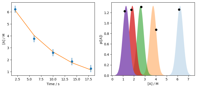
Therefore, the likelihood, \(p[D | M(\Theta)]\) is around 4.86. Let’s see how that looks on the data.

a_range = np.linspace(data['At'].min() - 1, data['At'].max() + 1, 1000)
fo = first_order(data['t'], *theta)

fig, ax = plt.subplots(1, 2, figsize=(10, 4))
ax[0].errorbar(data['t'], data['At'], data['At_err'], fmt='o')
ax[0].plot(data['t'], fo)
ax[0].set_xlabel('Time / s')
ax[0].set_ylabel('[A] / M')
[ax[1].fill_between(a_range, 
                    norm.pdf(a_range, data['At'][i], data['At_err'][i]), 
                    alpha=(i+1) / len(data)) for i in range(len(data))]
[ax[1].plot(f, d.pdf(f), 'ko') for d, f in zip(D, fo)]
ax[1].set_xlabel('[A] / M')
ax[1].set_ylabel('p([A])')
ax[1].set_ylim(0, None)
plt.show()

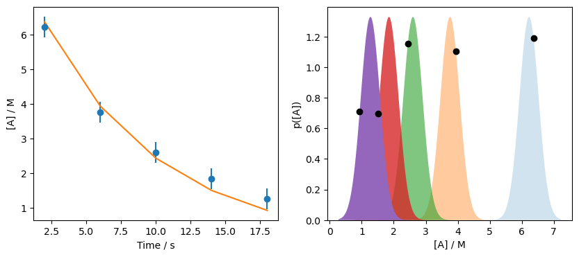
Once again, we do not maximise the likelihood of all distributions. Let’s try optimising \(\Theta\).

def negative_likelihood(theta):
    """
    The negative likelihood function for the first order rate equation.
    
    :param theta: The parameters to evaluate the negative likelihood at.
    
    :return: The negative likelihood at theta.
    """
    return -np.sum([d.pdf(first_order(t, theta[0], theta[1])) 
                    for d, t in zip(D, data['t'])])

res = minimize(negative_likelihood, [0.12, 8.1])
res.x

array([0.10459845, 7.55723452])

So the optimised parameters are about 0.10 and 7.56. We can plot these to see how we are doing.

a_range = np.linspace(data['At'].min() - 1, data['At'].max() + 1, 1000)
fo = first_order(data['t'], *res.x)

fig, ax = plt.subplots(1, 2, figsize=(10, 4))
ax[0].errorbar(data['t'], data['At'], data['At_err'], fmt='o')
ax[0].plot(data['t'], fo)
ax[0].set_xlabel('Time / s')
ax[0].set_ylabel('[A] / M')
[ax[1].fill_between(a_range, 
                    norm.pdf(a_range, data['At'][i], data['At_err'][i]),
                    alpha=(i+1) / len(data)) for i in range(len(data))]
[ax[1].plot(f, d.pdf(f), 'ko') for d, f in zip(D, fo)]
ax[1].set_xlabel('[A] / M')
ax[1].set_ylabel('p([A])')
ax[1].set_ylim(0, None)
plt.show()

This is a clear improvement, but we still don’t reach the maximum on all probability distributions. For example, consider the distribution centred on \([A]\) of 3.76, is it clear that the model has not maximised the distribution in this case. However, recall that we are working with the constraint of a model \(M\), hence the language “given model, \(M\), and parameters, \(\Theta\). No set of \(\Theta\) will fully maximise all of these distributions for the model \(M\), instead we find the value that give the best maximum, overall.

This is a very general approach to data analysis, and is closely related to the Bayesian modelling that we will look at later. However, you may notice that while we have optimised parameters, we don’t yet have information about the uncertainty in our model. This is what we will probe next.