Artificial Neurons

Like our neuron cells, an artificial neuron will allow the transmission of some signals only when some threshold, based on the inputs, is reached. In our artificial neutron, this threshold is known as a bias, \(b\). The inputs, \(x_n\), are the data that we input to the neuron, which are acted on by wights, \(w_n\), and combined in some transfer function, \(f(\mathbf{x}, \mathbf{w})\).

Comparison With the Biological Neuron

If we consider a biological neuron, this takes signals from the dendrites, which are connected to other neurons (the inputs). In the cell body, the signals are processed, and it is determined whether the neuron will fire an electrical signal. The processing involves weighting the signals based on the strength of the synaptic connections (this process is analogous to the weights and the transfer function). If the processing results in a signal being fired (an output), this is transmitted down the axon to be received by other neurons.

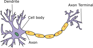
Fig. 35 A cartoon of a biological neuron with different, relevant components identified.

We can see a diagram of a single artificial neuron in Fig. 36 for comparison to a biological neuron.

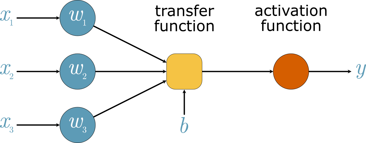
Fig. 36 A diagram of a single forward propagating artificial neuron would be a perceptron when the activation function is a Heaviside function.

Perceptron

The simplest form of an artificial neuron is the perceptron, which was first proposed in 1943 [12], and consists of just input and output layers (no hidden layers). In the perceptron algorithm, the transfer function is a simple summation, and the activation function is a Heaviside function, \(H(x)\). The Heaviside function has the following form,

\[\begin{split} H(x) := {\begin{cases} 1, & x\geq 0 \\ 0, & x<0 \end{cases}}, \end{split}\]

We can implement these in Python as follows:

import numpy as np
import matplotlib.pyplot as plt

def heaviside(x):
    """
    Heaviside step function.
    
    :param x: input value
    
    :return: 1 if x >= 0, 0 otherwise
    """
    return np.where(x < 0, 0, 1)

fig, ax = plt.subplots()

x = np.linspace(-5, 5, 100)

ax.plot(x, heaviside(x))
ax.set_xlabel('x')
ax.set_ylabel('H(x)')
plt.show()  

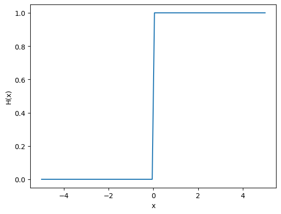
When \(x\) is a positive value, the return is 1, and 0 otherwise.

The AND Perceptron

We can use a simple perceptron to build logical operations, such as the AND operation. Consider a perceptron with two inputs, \(\mathbf{x} = \begin{bmatrix} x_1 \\ x_2 \end{bmatrix}\), therefore two weights, \(\mathbf{w} = \begin{bmatrix} w_1 \\ w_2 \end{bmatrix}\), and a bias, \(b\). We can define a truth table for the AND operation and the inputs \(x_1\) and \(x_2\), where 0 is equivalent to False and 1 to True.

Table 2 The truth table for the AND operation

\(x_1\)	\(x_2\)	AND output
0	0	0
1	0	0
0	1	0
1	1	1

If we now consider where \(\mathbf{w} = \begin{bmatrix} 1 \\ 1 \end{bmatrix}\), the result of the transfer function, a summation, is shown below for each of the pairs of \(x_1\) and \(x_2\).

Note

In the code here, we use np.dot, equivalent to \(\sum_{i=1}^{n}x_iw_i\). I told you linear algebra was going to be important for machine learning!

x = np.array([[0, 0],
              [0, 1],
              [1, 0],
              [1, 1]])
w = np.array([1, 1])

np.dot(x, w)

array([0, 1, 1, 2])

We know we want the first three sets of inputs to return 0 and the final to return 1. Therefore, we want the values going into the Heaviside to be less than 0 for the first three and more than 0 for the final. This means that the threshold to overcome should be that the result above is greater than one, and \(b\) should be in the range \(-2 < b < -1\). Below, we use \(b = -1.5\).

b = -1.5

heaviside(np.dot(x, w) + b)

array([0, 0, 0, 1])

The Problem of XOR

In 1969, Minksy and Papert [13] presented an elegant proof that a single-layer perceptron could not implement a simple XOR operation. The XOR, or eXclusive OR, operation can be thought of as the same as our linguistic or, i.e., “You can go up OR downstairs”; you cannot do both. Therefore, the truth table for XOR would look like the following.

Table 3 The truth table for the XOR operation

\(x_1\)	\(x_2\)	XOR output
0	0	0
1	0	1
0	1	1
1	1	0

In their book, Minsky and Papert imply that given that XOR logic cannot be implemented with a single-layer perceptron, larger networks will also have similar limitations and should be dropped. This significantly impacted artificial intelligence research, resulting in the AI winter that lasted until the early 1990s. However, as we will see, it is possible to implement the XOR operation with just a single hidden layer.