Nested Sampling

A popular and efficient algorithm to estimate the Bayesian evidence is known as nested sampling. Nested sampling was developed by the physicist John Skilling to improve the efficiency of Bayesian evidence estimation [11]. The nested sampling algorithm aims to transform a high-dimensional evidence integral—recalling that the dimensionality of the evidence integral is the same as the number of paramters—into a one-dimensional sum over likelihood values. The nested sampling algorithm is conceptually relatively simple. Initially, we will describe it by analogy.

Adventuring a Landscape

Consider a group of explorers investigating a mountainous landscape (the integral we want to compute). Instead of wandering randomly across the mountains (as in Markov chain Monte Carlo), nested sampling starts by placing a series of scouts randomly across the terrain (the placements are random samples from our priors). The scout in the lowest valley (the area of lowest probability) is replaced by a new one in a higher location. Over time, scouts climb higher and higher, focussing more and more on the landscape’s most important (highest probability) regions. In keeping track of how much area/volume is discarded at each step of the algorithm to build up an estimation of the total volume of the landscape, the Bayesian evidence integral.

The Algorithm

The nested sampling algorithm starts with a formulation of the Bayesian evidence integral,

\[ p(D | M) = \int p[D | M(\Theta)]p[M(\Theta)]\;\text{d}\Theta, \]

where \(p(D | M(\Theta))\) is the likelihood and \(p(M(\Theta))\) is the prior. We then introduce the prior volume*,

\[ X(\lambda) = \int_{p[D | M(\Theta)] > \lambda} p[M(\Theta)]\;\text{d}\Theta, \]

such that \(X(\lambda)\) represents the total prior mass where the likelihood is greater than \(\lambda\). From this, we can rewrite the evidence as,

\[ p(D | M) = \int_0^1 p(D | X)\;\text{d}X, \]

where, \(p(D | X)\) is the likelihood value corresponding to the prior volume \(X\).

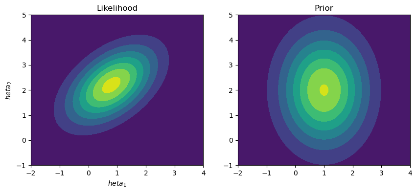
With the problem then reformulated, we can start to implement the algorithm. To achieve this, we are considering likelihood and prior functions that are both two-dimensional normal distributions over the parameters, \(\Theta = [\theta_1, \theta_2]\).

from scipy.stats import multivariate_normal as mv
from scipy.stats import norm
import matplotlib.pyplot as plt
import numpy as np

likelihood = mv(mean=[0.8, 2.2], cov=[[1, 0.5], [0.5, 1]])
priors = [norm(loc=1, scale=1), norm(loc=2, scale=1.5)]

x = np.linspace(-2, 4, 100)
y = np.linspace(-1, 5, 100)
X, Y = np.meshgrid(x, y)
pos = np.dstack((X, Y))
L_pdf = likelihood.pdf(pos)
P_pdf = priors[0].pdf(X) * priors[1].pdf(Y)

fig, ax = plt.subplots(1, 2, figsize=(10, 4))
ax[0].contourf(X, Y, L_pdf)
ax[0].set_title('Likelihood')
ax[0].set_xlabel('$\theta_1$')
ax[0].set_ylabel('$\theta_2$')
ax[1].contourf(X, Y, P_pdf)
ax[1].set_title('Prior')
ax[0].set_xlabel('$\theta_1$')
ax[0].set_ylabel('$\theta_2$')
plt.show()

Before we draw any samples, we set up the \(\ln\{p[D | M(\Theta)]\}\) that will be updated and gradually estimated using this algorithm.

Note

Recall the utility of logarithms in probabilistic sampling.

log_evidence = -np.inf

This starts with a value of the evidence of 0; hence, the logarithm is negative infinity.

Next, we create the initial prior volume, 1, as the prior is a normalised probability distribution, i.e., the integral is 1. We also define the number of samples or live points to be used.

N_samples = 1000
X = 1

With these aspects defined, we initialise our first samples.

samples = np.vstack([priors[0].rvs(N_samples), priors[1].rvs(N_samples)]).T

Then, we compute the likelihood for each of the samples.

samples_logl = likelihood.logpdf(samples)

Next, we update the logarithmic evidence with the worst log-likelihood, which will be discarded. We also remove the remove some section from the prior volume. Here, we take a naïve approach that assumes that the prior volume decreases following,

\[ X_i = X_{i-1} \exp(\frac{-1}{N}), \]

where \(i\) is the algorithm iteration and \(N\) is the number of samples.

X_new = X * np.exp(-1 / N_samples)
dX = X - X_new
X = X_new

change_in_log_evidence = samples_logl.min() + np.log(dX)
log_evidence = np.logaddexp(log_evidence, change_in_log_evidence)

Note the use of the np.logaddexp convince function. We can now look at the log_evidence

log_evidence

-29.364728250666325

Now, we must use some approach to update the samples, discarding the worst for a new sample with a higher likelihood. Here, we implement a naïve accept-reject step, where new samples are drawn until a better sample is found. Other approaches are more efficient but more complex to discuss, such as using an MCMC step.

def update_samples(sample, priors, likelihood):
    """
    Update the samples using the prior and likelihood.
    
    :param sample: the current samples
    :param prior: the prior distribution
    :param likelihood: the likelihood distribution
    
    :return: New updated samples
    """
    samples_logl = likelihood.logpdf(samples)
    min_likelihood = samples_logl.min()
    new_sample = np.array([priors[0].rvs(1), priors[0].rvs(1)]).flatten()
    new_likelihood = likelihood.pdf(new_sample)
    while min_likelihood > new_likelihood:
        new_sample = np.array([priors[0].rvs(1), priors[0].rvs(1)]).flatten()
        new_likelihood = likelihood.pdf(new_sample)
    samples[samples_logl.argmin()] = new_sample
    return samples

samples = update_samples(samples, priors, likelihood)

We can then construct this process into a loop with some stopping criteria. A standard stopping criterion is when very little change in the log evidence is observed with each additional iteration.

log_evidence_list = []

while change_in_log_evidence > -100:
    samples_logl = likelihood.logpdf(samples)

    dX = X / N_samples
    X -= dX

    change_in_log_evidence = samples_logl.min() + np.log(dX)
    log_evidence_list.append(log_evidence)
    log_evidence = np.logaddexp(log_evidence, change_in_log_evidence)
    samples = update_samples(samples, priors, likelihood)

log_evidence

-3.909274999881445

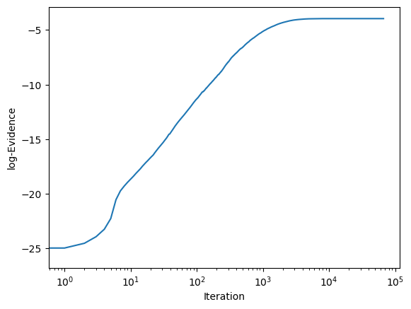
We can then visualise the log evidence as a function of iteration to check the convergence.

fig, ax = plt.subplots()

ax.plot(log_evidence_list)
ax.set_ylabel('log-Evidence')
ax.set_xlabel('Iteration')
ax.set_xscale('log')
plt.show()

Similar to many of the algorithms we have looked at, using an existing, more complete implementation is more effective than one we write ourselves. Therefore, let’s look at using the ultranest package.