Recurrent Neural Networks#
The neural networks we have investigated are sometimes called feedforward neural networks. These types of neural networks can be limited as the inputs are all processed independently by the network. The independence is addressed with recurrent neural networks, where the output of a neuron for a given data point is fed in as an input for the following data point. This makes recurrent neural networks uniquely suited for modelling sequential data, such as text, speech and time series. As a result, recurrent neural networks have significantly influenced the transformer networks that have led to the revolutionary large language models.
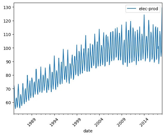
We will use a simple time series dataset for the electrical production to put together a simple recurrent neural network. You can download the dataset here.
import pandas as pd
import matplotlib.pyplot as plt

timeseries = pd.read_csv('../data/electric.csv')
timeseries['date'] = pd.to_datetime(timeseries['date'])

fig, ax = plt.subplots()
timeseries.plot(x='date', y='elec-prod', ax=ax)
ax.tick_params(axis='x', labelrotation=45)
plt.show()
Feedback#
As mentioned above, the difference between a traditional neural network and a recurrent neural network is that the latter includes the hidden state of the previous data point in the activation function. That means that for some activation function, \(f\), the traditional network as the equation,
while for a recurrent network, we add the previous hidden state,
We implement a simple feedback perceptron with Python below, using a tanh activation function.
import numpy as np

class SimpleRNNPerceptron:
    """
    A simple RNN perceptron with a single hidden layer.

    :param input_size: The size of the input vector
    :param hidden_size: The size of the hidden layer
    """
    def __init__(self, input_size, hidden_size):
        self.hidden_size = hidden_size

        self.W_x = np.random.randn(hidden_size, input_size) * 0.1
        self.W_h = np.random.randn(hidden_size, hidden_size) * 0.1
        self.b = np.zeros((hidden_size, 1))
        self.h_i = np.zeros((hidden_size, 1))

    def step(self, x_i):
        """
        Processes a single step

        :param x_i: The input vector
        :return: The output vector
        """
        x_i = x_i.reshape(-1, 1)
        self.h_i = np.tanh(np.dot(self.W_x, x_i) + np.dot(self.W_h, self.h_i) + self.b)
        return self.h_i

rnn = SimpleRNNPerceptron(input_size=1, hidden_size=5)
We can run this through a single year of our time series data, where the hidden size is 5. The hidden size is the number of neurons in the hidden layer.
timeseries_2017 = timeseries['elec-prod'][timeseries['date'].dt.year == 2017]
timeseries_2017 /= timeseries_2017.max()

for i, x_i in enumerate(timeseries_2017):
    h_i = rnn.step(np.array([x_i]))
    print(f"Step {i+1}: Hidden State = {h_i.ravel()}")
Step 1: Hidden State = [ 0.16710018  0.02078055 -0.0111547   0.07660058  0.0180928 ]
Step 2: Hidden State = [0.12398451 0.05142897 0.01316723 0.04522538 0.00318047]
Step 3: Hidden State = [0.12210037 0.0450257  0.002063   0.05191576 0.01308904]
Step 4: Hidden State = [0.10702724 0.04188691 0.00433163 0.04344852 0.00918468]
Step 5: Hidden State = [0.11423646 0.03945036 0.00201827 0.0478988  0.01102148]
Step 6: Hidden State = [0.12878497 0.04257764 0.0024701  0.05368667 0.01144781]
Step 7: Hidden State = [0.1408991  0.04736505 0.00326273 0.05852978 0.01225292]
Step 8: Hidden State = [0.1339347  0.04938038 0.00478079 0.05485533 0.01136679]
Step 9: Hidden State = [0.11926093 0.04626147 0.004467   0.04885928 0.01070395]
Step 10: Hidden State = [0.11431114 0.04234151 0.00316656 0.04736392 0.01072847]
Step 11: Hidden State = [0.12114148 0.04185121 0.00257883 0.05046545 0.01114299]
Step 12: Hidden State = [0.14559147 0.04630176 0.00197172 0.06119374 0.01320832]
The larger the hidden size, the more capacity the network has to learn complex patterns, which comes with a computational cost.
Implementation with pytorch#
The Python library pytorch comes with an implementation of recurrent neural networks.
We advise you to study the documentation to understand how a recurrent neural network may be implemented using pytorch.
Furthermore, you should appreciate the configurability of this nn.Module object.