Computing the Posterior#
Previously, we discussed how to compute the likelihood and the probability of observing some data given a model and parameters, and we have now seen how to propose a prior probability. Therefore, if we look at Bayes’ theorem again, we can start to look at the so-called posterior.
the posterior is \(p(A | B)\), the conditional probability that we are trying to compute. However, we have not yet covered how to compute Bayes’ theorem’s denominator, known as the evidence term.
Sampling Parameters#
If we rewrite Bayes’ theorem in the notation of our data, \(D\), model, \(M\), and parameters, \(\Theta\), we get the following relation,
Our Bayesian analysis with the above equation usually aims to understand the distribution of the parameters, \(\Theta\). We note that \(\Theta\) does not appear in the denominator; therefore, changing the value of \(\Theta\) does not affect this. This makes the denominator simply a scaling factor, so we rewrite Eqn. (39) as,
Therefore, in sampling and maximising \(p[M(\Theta) | D]\), it is not necessary to compute the denominator. We can now look at using PyMC to achieve this. Let’s load in the chemical data we have seen previously.
import pandas as pd
import numpy as np
from scipy.stats import norm

data = pd.read_csv('../data/first-order.csv')

D = [norm(data['At'][i], data['At_err'][i]) for i in range(len(data))]

def first_order(t, k, A0):
    """
    A first order rate equation.

    :param t: The time to evaluate the rate equation at.
    :param k: The rate constant.
    :param A0: The initial concentration of A.

    :return: The concentration of A at time t.
    """
    return A0 * np.exp(-k * t)
The only change necessary is to use the informative prior in the pm.Model.
This is because PyMC always performs posterior sampling; it is just that the use of an uninformative prior (the uniform distribution) is numerically equivalent to sampling just the likelihood.
import pymc as pm

with pm.Model() as model:
    k = pm.Normal('k', 0.15, 0.01)
    A0 = pm.Normal('A0', 7.5, 0.5)

    At = pm.Normal('At',
                   mu=first_order(data['t'], k, A0),
                   sigma=data['At_err'],
                   observed=data['At'])

    trace = pm.sample(1000, tune=1000, chains=10, progressbar=False)
/usr/share/miniconda/envs/special-topics/lib/python3.11/site-packages/arviz/__init__.py:50: FutureWarning:
ArviZ is undergoing a major refactor to improve flexibility and extensibility while maintaining a user-friendly interface.
Some upcoming changes may be backward incompatible.
For details and migration guidance, visit: https://python.arviz.org/en/latest/user_guide/migration_guide.html
  warn(
Initializing NUTS using jitter+adapt_diag...
Multiprocess sampling (10 chains in 2 jobs)
NUTS: [k, A0]
Sampling 10 chains for 1_000 tune and 1_000 draw iterations (10_000 + 10_000 draws total) took 5 seconds.
Again, we can visualise the traces using arviz.
import matplotlib.pyplot as plt
import arviz as az

az.plot_trace(trace, var_names=["k", "A0"])
plt.tight_layout()
plt.show()
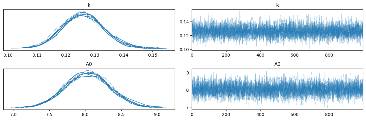
By comparing this to the likelihood sampling result, we can see the influence of the priors and Bayes’ theorem. It is important to highlight that we are computing the probability of the model, Eqn, (38) here, with the parameters above given the data, instead of the probability that data, \(D\), would be observed given some model, which was what was computed in the likelihood sampling.