Policy Search

The training of a reinforcement learning loop is a process that aims to generate a policy that leads to the reward being maximised. This is an optimisation process; instead of optimising specific values, we are trying to optimise the policy defining the action. It is easiest to imagine this policy as a discrete variable to be optimised, i.e., should the policy be policy A or policy B. However, if we break the policy down into constituent parts, we can see the continuous nature of the problem. Consider the robot vacuum example; there are two parameters that can be controlled: how large the rotations of the vacuum are (\(r\)) and how frequently it does so (\(p\)). This is shown visually for a few positions in policy space in vacuum.

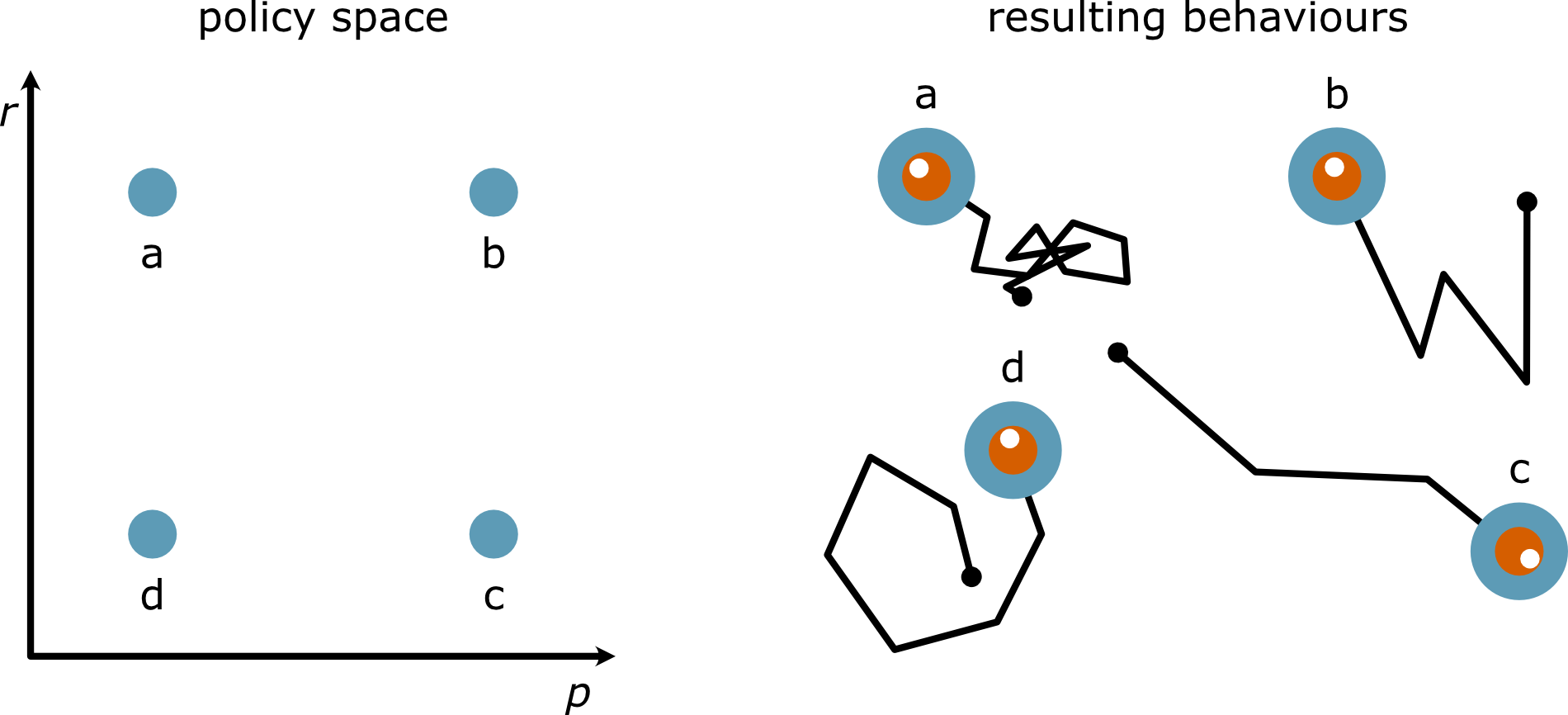
Fig. 42 Some examples of policies may be found in the example of a robot vacuum.

Let’s consider two possible policies for the LunarLander-v3 environment. One will be the modulo example used before, and the other will be a more logical approach, where the lunar is moved left or right based on the position in the x dimension and the downward thruster is only used when the y velocity is greater than some threshold.

def modulo_policy(step, obs):
    """
    Returns and action based on the modulo of the step in the episode.
    
    :param step: The step in the episode.
    :return: The action to take.
    """
    return step % 4

def logical_policy(step, obs):
    """
    A more logical policy that takes into account the observation.
    
    :param obs: The observation.
    :return: The action to take.
    """
    x_pos = obs[0]
    y_vel = obs[3]
    if y_vel < -0.4:
        return 2
    elif x_pos < -0.1:
        return 3
    elif x_pos > 0.1:
        return 1
    else:
        return 0
    

We can now compare the two policies, over 500 episodes of the LunarLander-v3, to see which performs best.

import gymnasium as gym
import numpy as np

env = gym.make('LunarLander-v3', render_mode='rgb_array')

policies = [modulo_policy, logical_policy]
total_rewards = np.zeros((2, 500))
render = [None, None]
for i, policy in enumerate(policies):
    for repeat in range(total_rewards.shape[1]):
        current_rewards = 0
        obs = env.reset()[0]
        current_render = []
        for step in range(env.spec.max_episode_steps):
            action = policy(step, obs)
            obs, reward, terminated, truncated, info = env.step(action)
            current_rewards += reward
            current_render.append(env.render())
            if terminated:
                break
        if current_rewards > total_rewards[i].max():
            render[i] = current_render
        total_rewards[i, repeat] = current_rewards

        env.close()

We can now compare the total reward from each episode.

import matplotlib.pyplot as plt

fig, ax = plt.subplots()

ax.hist(total_rewards[0], label='Modulo Policy', density=True)
ax.hist(total_rewards[1], label='Logical Policy', density=True)
ax.legend()
ax.set_xlabel('Reward')
ax.set_ylabel('p(Reward)')
plt.show()

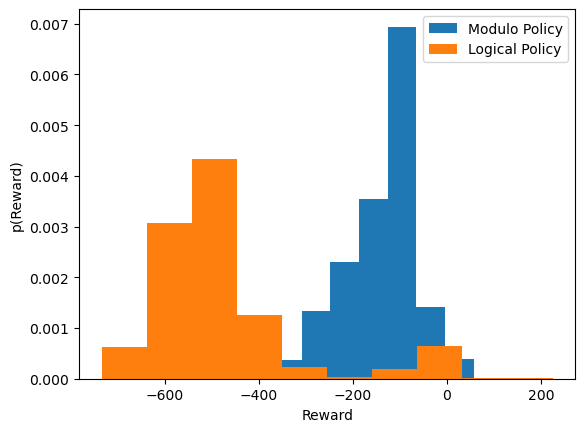
It can be seen that the modulo policy, on average, does better than the logical policy in this case. However, the logical policy follows a bimodal distribution, so with some tuning, it could potentially outperform the modulo policy.

We will save these rewards for use later.

np.savetxt('total_rewards.txt', total_rewards)