Using t-SNE in Practice

Previously, we looked at the details of how the t-SNE algorithm works. However, as with many things in data science, the t-SNE algorithm has already been implemented in existing software. Specifically, we will look at using t-SNE from scikit-learn. We will look at how t-SNE handles the MNIST handwritten digits data, so let’s start by reading that file.

import pandas as pd

data = pd.read_csv('./../data/mnist.csv')

Instead of working with the entire dataset, we will take just a subsample of the data and work with that. This will help our t-SNE algorithm run a bit faster.

subsample = data.sample(n=1000, random_state=42)
subsample

	pixel1	pixel2	pixel3	pixel4	pixel5	pixel6	pixel7	pixel8	pixel9	pixel10	...	pixel776	pixel777	pixel778	pixel779	pixel780	pixel781	pixel782	pixel783	pixel784	label
10650	0	0	0	0	0	0	0	0	0	0	...	0	0	0	0	0	0	0	0	0	6
2041	0	0	0	0	0	0	0	0	0	0	...	0	0	0	0	0	0	0	0	0	9
8668	0	0	0	0	0	0	0	0	0	0	...	0	0	0	0	0	0	0	0	0	5
1114	0	0	0	0	0	0	0	0	0	0	...	0	0	0	0	0	0	0	0	0	7
13902	0	0	0	0	0	0	0	0	0	0	...	0	0	0	0	0	0	0	0	0	4
...	...	...	...	...	...	...	...	...	...	...	...	...	...	...	...	...	...	...	...	...	...
7683	0	0	0	0	0	0	0	0	0	0	...	0	0	0	0	0	0	0	0	0	9
17821	0	0	0	0	0	0	0	0	0	0	...	0	0	0	0	0	0	0	0	0	2
10261	0	0	0	0	0	0	0	0	0	0	...	0	0	0	0	0	0	0	0	0	0
12964	0	0	0	0	0	0	0	0	0	0	...	0	0	0	0	0	0	0	0	0	6
88	0	0	0	0	0	0	0	0	0	0	...	0	0	0	0	0	0	0	0	0	0

1000 rows × 785 columns

Hyperparameters of t-SNE

Unlike PCA, t-SNE has some so-called hyperparameters that can be used to control algorithm implementation. We have already met one of these, but we will highlight a few others in this section.

Perplexity

We will start by looking at the effect of changing the perplexity on the results from t-SNE. When discussing the algorithm, it was mentioned that the perplexity balances between the local and global structure. Let’s start with the default value for the TSNE object from scikit-learn, which is 30.

from sklearn.manifold import TSNE

def control_hyperparameters(perplexity=30, learning_rate='auto', early_exaggeration=12):
    """
    A helper function to control hyperparameters of t-SNE.
    """
    dataset = subsample.copy()
    tsne = TSNE(n_components=2, 
                perplexity=perplexity, 
                learning_rate=learning_rate, 
                early_exaggeration=early_exaggeration, 
                random_state=42)
    tsne_result = tsne.fit_transform(dataset.drop('label', axis=1))
    dataset['tSNE1'] = tsne_result[:, 0]
    dataset['tSNE2'] = tsne_result[:, 1]
    return dataset

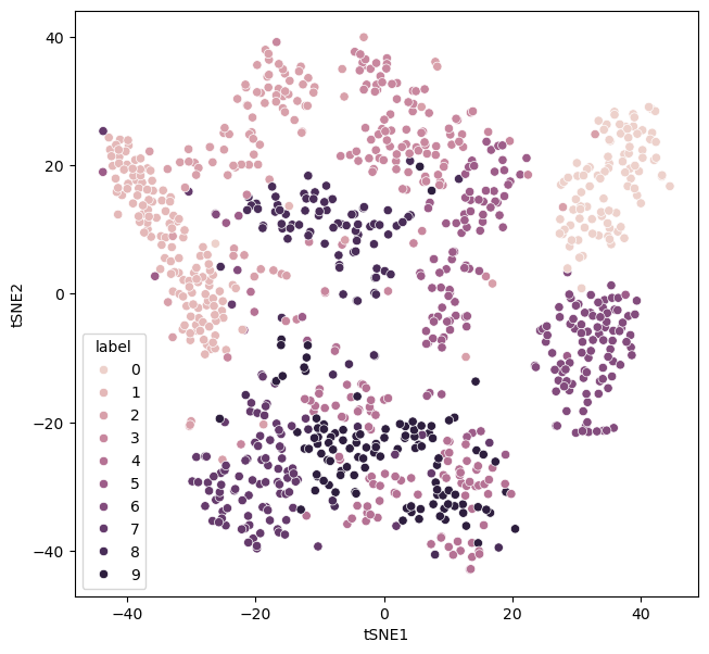
perplexity_30 = control_hyperparameters(perplexity=30)

The above function can be reused to test different values. Let’s look at how the data are distributed with a perplexity of 30.

import matplotlib.pyplot as plt
import seaborn as sns

fig, ax = plt.subplots(figsize=(9, 7))
sns.scatterplot(x='tSNE1', y='tSNE2', hue='label', legend='full', data=perplexity_30, ax=ax)
ax.set_aspect('equal')
plt.show()

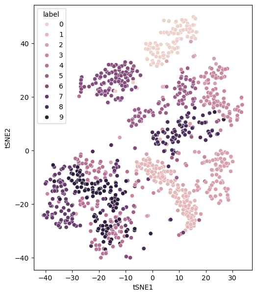
There are some clear clusters of given numbers. A low perplexity value is associated with local structure over global structure. However, for extremely small values of perplexity, this can lead to many small clusters. Consider a perplexity of the value of 1.

perplexity_1 = control_hyperparameters(perplexity=1)
fig, ax = plt.subplots(figsize=(9, 7))
sns.scatterplot(x='tSNE1', y='tSNE2', hue='label', legend='full', data=perplexity_1, ax=ax)
ax.set_aspect('equal')
plt.show()

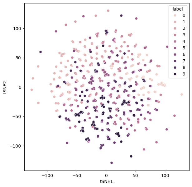
Meanwhile, a large perplexity value prioritises the global structure over the local. Again, this can have undesirable results for extreme values – producing data lacks structure.

perplexity_600 = control_hyperparameters(perplexity=600)
fig, ax = plt.subplots(figsize=(9, 7))
sns.scatterplot(x='tSNE1', y='tSNE2', hue='label', legend='full', data=perplexity_600, ax=ax)
ax.set_aspect('equal')
plt.show()

The perplexity is probably the most important hyperparameter in the use of t-SNE. Unfortunately, there is no simple rule for selecting the value of perplexity. Generally, the best advice is to test a few different values and decide which value leads to the most informative transformed data for the problem at hand.

Learning Rate

The learning rate affects the algorithm used to minimise the KL divergence. High learning rates can lead to faster convergence but may overshoot the minimum or cause instability.

perplexity_1 = control_hyperparameters(learning_rate=5000)
fig, ax = plt.subplots(figsize=(9, 7))
sns.scatterplot(x='tSNE1', y='tSNE2', hue='label', legend='full', data=perplexity_1, ax=ax)
ax.set_aspect('equal')
plt.show()

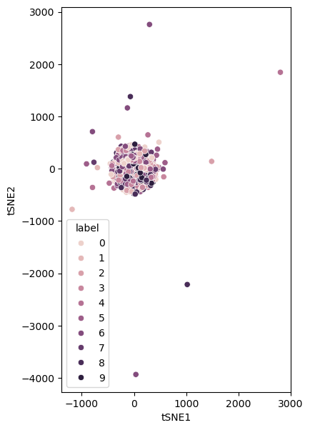
A low learning rate will lead to a very slow convergence.

Early Exaggeration

Another hyperparameter that impacts the minimisation process it the early exaggeration. This involves exaggerating the affinities in high dimensional space during the initial stages of the algorithm. This can be important in creating more meaningful clusters.

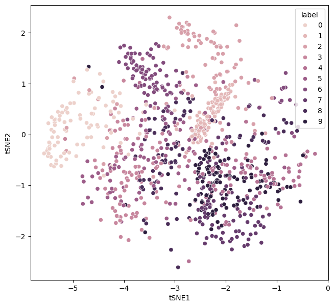
We can see the impact of no early exaggeration for the MNIST dataset below.

perplexity_1 = control_hyperparameters(early_exaggeration=1)
fig, ax = plt.subplots(figsize=(9, 7))
sns.scatterplot(x='tSNE1', y='tSNE2', hue='label', legend='full', data=perplexity_1, ax=ax)
ax.set_aspect('equal')
plt.show()