DBSCAN

Density-Based Spatial Clustering of Applications with Noise, or DBSCAN for short, is an algorithm that groups data points in areas of high density and then identifies data in lower-density regions as noise. Similar to the purely hierarchical clustering method discussed previously, this does not assume the shape of the clusters. Unlike k-means and GMMs, which assume spheres and ellipses, respectively. Additionally, it does not assume some given cluster number.

To discuss the DBSCAN algorithm, let’s look at a slightly different dataset.

import numpy as np
import matplotlib.pyplot as plt

X = np.loadtxt('../data/moons_blobs.txt') 

fig, ax = plt.subplots(figsize=(4, 4))
ax.plot(*X.T, '.')
ax.axis('equal')
plt.show()

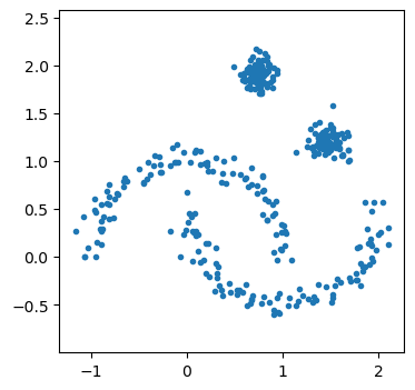
We see that there are four clusters, two of which are intersecting moons and two are circular. First, we can see how GMMs would cope.

from sklearn.mixture import GaussianMixture

gmm = GaussianMixture(n_components=4, random_state=42)
gmm.fit(X)
label = gmm.predict(X)
prob = gmm.predict_proba(X)
size = 50 * prob.max(1) ** 2

fig, ax = plt.subplots(figsize=(4, 4))
ax.scatter(*X.T, s=size, c=label)
ax.axis('equal')
plt.show()

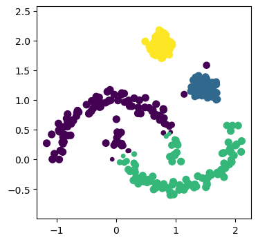
It is clear that even though the Gaussian mixture model is told that there are 4 clusters, it fails to find the moons, given they cannot be described with an elliptical model. However, can the DBSCAN approach improve on this?

DBSCAN Algorithm

We will need to know the distance between all the points. So, let’s generate that in the same fashion as previously.

from scipy.spatial.distance import pdist, squareform

distances = squareform(pdist(X))
np.fill_diagonal(distances, np.inf)

At the algorithm’s start, all data points are classified as unvisited.

visited = [False] * X.shape[0]

We will then visit the first data point and update the visited status.

visited[0] = True

For that first data point, we want to find all of the other points that are less than some distance eps from it; these are the neighbours of the data point. This eps is one of the hyperparameters of the DBSCAN algorithm; for this example, we will use a value of 0.1.

eps = 0.1
np.where(distances[0] < eps)

(array([ 57, 186]),)

Note

This classification as noise may change in the future.

If the data point has fewer than min_samples (the second hyperparameter, here we use 5), then it is identified as noise. We will do this by making the value of a labels array -1.

min_samples = 5
labels = np.zeros(X.shape[0], dtype=int)

if (distances[0] < eps).sum() < min_samples:
    labels[0] = -1

However, if the point has more than min_samples neighbours, we classify it as a core point and expand the cluster around it. Data point 338 has many neighbours.

(distances[338] < eps).sum()

49

A core point is assigned a cluster_id, which starts from 0.

cluster_id = 0

labels[338] = cluster_id

And then, for each point in the neighbour of a data point, we perform the following:

• If the point is unvisited, its neighbours are found and marked as visited, and if it has more than the min_samples of neighbours, then these are included as neighbours of the core point.

• If the point has been visited and is currently defined as noise, the label is changed to that of the core point.

This is shown for data point 338 below.

neighbours = np.where(distances[338] < eps)[0]

j = 0
while j < neighbours.size:
    current = neighbours[j]
    if not visited[current]:
        visited[current] = True
        new_neighbors = np.where(distances[current] <= eps)[0]
        if new_neighbors.size >= min_samples:
            neighbours = np.concatenate([neighbours, new_neighbors])
    if labels[current] == -1:
        labels[current] = cluster_id
    j += 1
cluster_id += 1

We can see that this has led to many particles being visited.

np.sum(visited)

98

To put the algorithm together, we will reset some of the bookkeeping.

visited = [False] * X.shape[0]
labels = np.zeros(X.shape[0], dtype=int) - 1
cluster_id = 0

for i in range(X.shape[0]):
    if not visited[i]:
        visited[i] = True
        neighbours = np.where(distances[i] <= eps)[0]
        if neighbours.size < min_samples:
            labels[i] = -1
        else:
            labels[i] = cluster_id
            j = 0
            while j < neighbours.size:
                current = neighbours[j]
                if not visited[current]:
                    visited[current] = True
                    new_neighbors = np.where(distances[current] <= eps)[0]
                    if new_neighbors.size >= min_samples:
                        neighbours = np.concatenate([neighbours, new_neighbors])
                if labels[current] == -1:
                    labels[current] = cluster_id
                j += 1
            cluster_id += 1

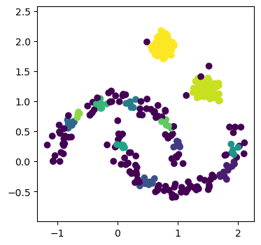
Using the current hyperparameter values, the DBSCAN algorithm has produced 12 clusters.

np.unique(labels)

array([-1,  0,  1,  2,  3,  4,  5,  6,  7,  8,  9, 10, 11])

And identified 134 of the 400 data points as noise.

(labels == -1).sum()

134

We can try to visualise this, but there probably isn’t enough colour fidelity in the matplotlib standard plotting.

fig, ax = plt.subplots(figsize=(4, 4))
ax.scatter(*X.T, c=labels)
ax.axis('equal')

(-1.326488757153794,
 2.2672553780080644,
 -0.7370806052205164,
 2.3120420120835234)

HDBSCAN

Before we leave clustering behind, we will look at one final approach, Hierarchical DBSCAN[3]. HDBSCAN brings the hierarchical clustering approach together with DBSCAN. One of the significant benefits of HDBSCAN over DBSCAN is that it is not necessary to define the hyperparameters.

from sklearn.cluster import HDBSCAN

hdbscan = HDBSCAN()
label = hdbscan.fit_predict(X)

fig, ax = plt.subplots(figsize=(4, 4))
ax.scatter(*X.T, c=label)
ax.axis('equal')

(-1.326488757153794,
 2.2672553780080644,
 -0.7370806052205164,
 2.3120420120835234)

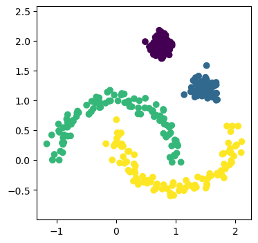
A naïve usage of the scipy.cluster.HBDSCAN method can perfectly capture the data.

This isn’t to say that HDBSCAN is perfect, but there is still room for other clustering methods. This is not least due to the high computational cost of HDBSCAN compared to the more straightforward approaches.