Hierarchical Clustering

Building a hierarchy of clusters can be beneficial to understanding the similarity between data points. Hierarchical clustering is a class of clustering methods that do not require the number of clusters at the time of analysis but instead allow the flexibility to choose the cluster numbers after the analysis is complete. Additionally, some argue that greater insight can be obtained from hierarchical clustering, which allows nested clusters to be found, revealing more information about the relationships between data points. A notable difference between hierarchical clustering and the previous clustering approaches discussed is that there is no underlying statistical model in hierarchical clustering as in the other approaches; i.e., we can think of k-means as a non-covariant equivalent to Gaussian mixture models.

Hierarchical clustering comes in two flavours:

• Agglomerative (or bottom-up) clustering starts with each data point as its own cluster and then merges nearby clusters. That approach is quite natural and intuitive.

• Divisive (or top-down) clustering does the opposite, recursively splitting clusters until some stopping criterion is reached. This is a less common approach due to increased computational complexity.

How Agglomerative Clustering Works

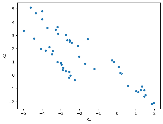
Here, we will look at agglomerative clustering in detail and build a simple example. We will use a subset of the dataset that k-means could not cluster correctly.

import numpy as np
import pandas as pd
import seaborn as sns
import matplotlib.pyplot as plt
from sklearn import datasets

data = pd.read_csv('../data/skew-small.csv')
X = data.values

fig, ax = plt.subplots()
sns.scatterplot(x='x1', y='x2', data=data, ax=ax)
plt.show()

The first step is to compute the distance matrix, all pairwise distances, between data points. We can achieve this with NumPy and using the np.newaxis functionality, but here we use functionality from the scipy.spatial.distance library. We also fill the diagonal with infinity values, representing the distance between a data point and itself, which is 0.

Note

pdist stands for pairwise distances and squareform produces an \(N\timesN\) matrix, where \(N\) is the number of data points.

from scipy.spatial.distance import pdist, squareform

distances = squareform(pdist(X))
np.fill_diagonal(distances, np.inf)

A Comment on Distance

The distance we traditionally calculate is the Euclidean distance between two points. However, in machine learning methods, other distance metrics can be used. Fig. 25 shows some of the other distances that are used.

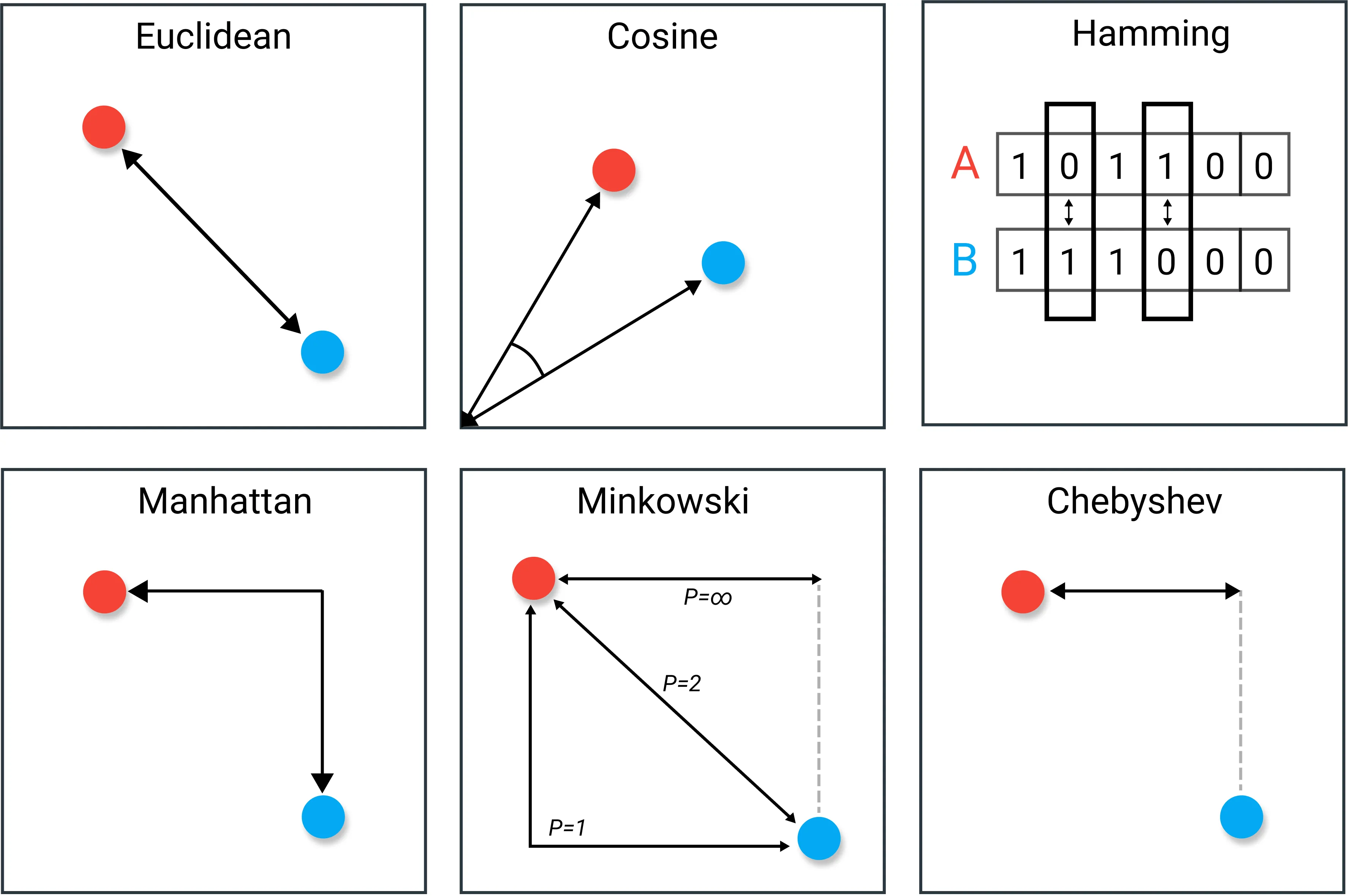
Fig. 25 A diagram presenting some different distances that may be used. Modified from Maatren Grootendorst.

The distance used must have a logical rationale behind it. A complete list of the distances that the scipy.spatial.distance.pdist function can compute can be found in the documentation.

Next, we start by creating a dictionary of clusters, where each point is its own cluster and create an empty list that we will use to store the dendrogram.

clusters = {i: [i] for i in range(X.shape[0])}
dendrogram = []

The next step is to find the two particles closest to each other.

distances.min()

0.06205110185796799

Two data points are only 0.062 away from each other. But which data points are they? We can find this by comparing the minimum of the newly created active_distances array with the distances array. This slightly convoluted approach is necessary, as we will remove rows and columns from the active_distances later, but to keep track of the indices, they won’t be removed from distances.

active_distances = distances.copy()
minimum_pair = np.array(np.where(distances == active_distances.min()))[:, 0]
minimum_pair

array([ 0, 17])

The two closest points are data point 0 and data point 17. Let’s check this.

fig, ax = plt.subplots()
sns.scatterplot(x='x1', y='x2', data=data, ax=ax)
ax.plot(X[[minimum_pair], 0], X[[minimum_pair], 1], 'ks')
plt.show()

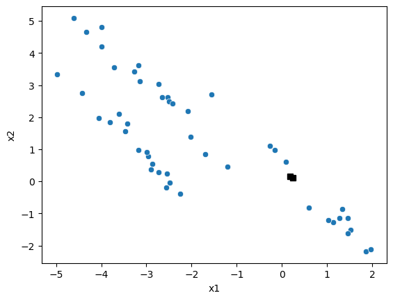
This looks correct, so we can now add our first cluster to the dendrogram.

dendrogram.append([minimum_pair[0], minimum_pair[1], active_distances.min(), len(clusters[minimum_pair[0]]) + len(clusters[minimum_pair[1]])])
new_cluster = clusters[minimum_pair[0]] + clusters[minimum_pair[1]]

The new_cluster replaces the first point in the dictionary, and we delete the second; this is essential bookkeeping.

del clusters[minimum_pair[1]]
clusters[minimum_pair[0]] = new_cluster

Next, we update the distance matrix. This involves finding the minimum distance between the two data points in the cluster and all the other data points (or clusters). This minimum distance is used to update the distance matrix.

for k in clusters.keys():
    distances[minimum_pair[0], k] = np.min([distances[p1, p2] for p1 in clusters[minimum_pair[0]] for p2 in clusters[k]])
    distances[k, minimum_pair[0]] = distances[minimum_pair[0], k]
distances[minimum_pair[0], minimum_pair[0]] = np.inf

The final step to update the distance matrix is to remove the rows and columns associated with the second cluster of the minimum pair. This is achieved by making a nested list of the indices in clusters and flattening this; the flattened list is then used in the np.delete function.

to_remove = [i for sublist in [v[1:] for k, v in clusters.items() if len(v) > 1] for i in sublist]

active_distances = distances.copy()
active_distances = np.delete(active_distances, to_remove, axis=0)
active_distances = np.delete(active_distances, to_remove, axis=1)

Again, this convoluted approach is necessary for clusters of clusters to be accounted for.

Linkages

Above, we use what is known as a single linkage criterion when we take the minimum distance of the points in the cluster from the other points. This is not the only approach to describe our clusters. Other linkages include:

• Complete linkage: where the maximum distance of the points in the cluster is used.

• Average linkage: where the average distance is used.

• Ward’s linkage[2]: looks to merge the clusters by minimising the total within-cluster variance.

The process is then repeated until there is only a single cluster.

clusters_list = [clusters.copy()]
while len(clusters) > 1:
    minimum_pair = np.array(np.where(distances == active_distances.min()))[:, 0]
    dendrogram.append([minimum_pair[0], minimum_pair[1], active_distances.min(), len(clusters[minimum_pair[0]]) + len(clusters[minimum_pair[1]])])
    new_cluster = clusters[minimum_pair[0]] + clusters[minimum_pair[1]]
    del clusters[minimum_pair[1]]
    clusters[minimum_pair[0]] = new_cluster 
    clusters_list.append(clusters.copy())
    for k in clusters.keys():
        distances[minimum_pair[0], k] = np.min([distances[p1, p2] for p1 in clusters[minimum_pair[0]] for p2 in clusters[k]])
        distances[k, minimum_pair[0]] = distances[minimum_pair[0], k]
    distances[minimum_pair[0], minimum_pair[0]] = np.inf
    to_remove = [i for sublist in [v[1:] for k, v in clusters.items() if len(v) > 1] for i in sublist]
    active_distances = distances.copy()
    active_distances = np.delete(active_distances, to_remove, axis=0)
    active_distances = np.delete(active_distances, to_remove, axis=1)

Visualisation of Hierarchical Clustering

Now that we have performed the hierarchical clustering, it is time to visualise the results. First of all, let’s look at the data with colours based on the clusters that have been assigned. We can do this for any number of clusters.

fig, ax = plt.subplots(1, 3, figsize=(15, 4))

for i, clusters in enumerate([2, 3, 4]):
    for k, v in clusters_list[-clusters].items():
        ax[i].scatter(X[v, 0], X[v, 1], label=k)
        ax[i].set_xlabel('x1')
        ax[i].set_ylabel('x2')
        ax[i].set_title(f'Clusters: {clusters}')
plt.show()

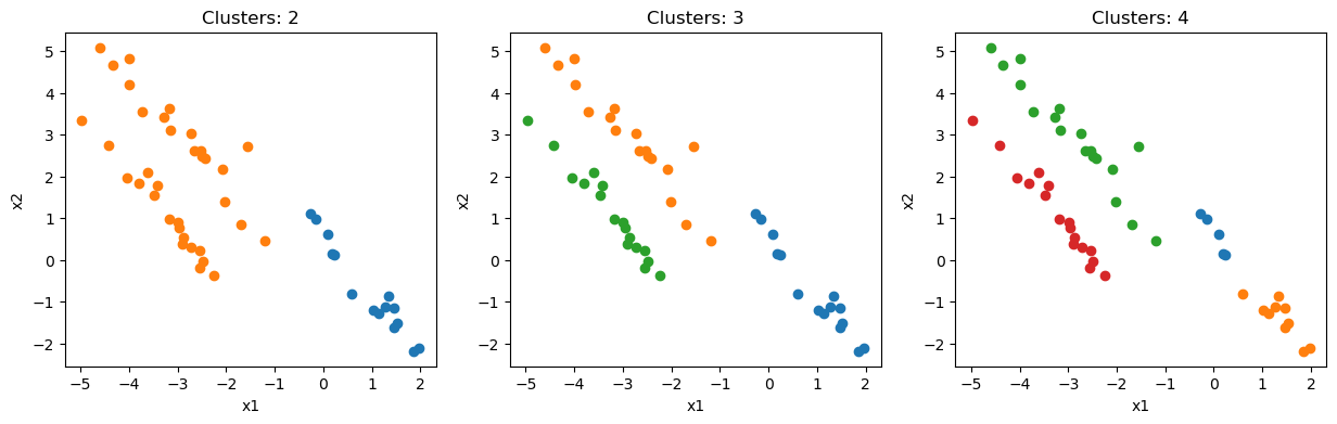
Unsurprisingly, three clusters are the best representation of the data. However, four is also quite convincing.

The following visualisation we can use can help us understand the groupings in our hierarchical clustering. This is called a dendrogram and represents the connectivity of the clusters at each step of the algorithm.

Note

We use a function from scipy.cluster.hierarchy to plot the dendrogram. However, this function’s expected input is slightly different from the dendrogram object we created in the algorithm. Therefore, a helper module can be used to convert to a compatible structure. The helper module can be downloaded here.

from scipy.cluster.hierarchy import dendrogram as dendrogram_plot
from helper import dendrogram_convert

dg = dendrogram_plot(dendrogram_convert(dendrogram))

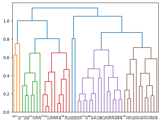
The dendrogram lets us see the connectivity but can also be used to determine how many clusters are meaningful. The areas with the largest vertical distance represent places where clusters very far apart have been linked. Hence, there is a large distance between four clusters (around 1 on the y-axis) and five clusters (around 0.87 on the y-axis).