Build Your Own#
Practically, writing a complex artificial neural network from scratch is inefficient.
This is particularly the case when we are working in Python, which has a broad range of tooling that covers neural network machine learning.
Instead, we will look at using pytorch to create our neural network.
We will start by importing pytorch.
import torch
Loading Data#
For this example, we will use the FashionMNIST dataset, which has 70 000 examples of images of clothes. Each of the images has been labelled with the type of clothing. Below, we list all of the classes.
classes = [
    "T-shirt/top",
    "Trouser",
    "Pullover",
    "Dress",
    "Coat",
    "Sandal",
    "Shirt",
    "Sneaker",
    "Bag",
    "Ankle boot",
]
This is split into a train and a test dataset; we will download these datasets from the torchvision.
from torchvision import datasets
from torchvision.transforms import ToTensor
from IPython.utils import io

with io.capture_output() as captured:
    training_data = datasets.FashionMNIST(
        root="../data",
        train=True,
        download=True,
        transform=ToTensor(),
    )

    test_data = datasets.FashionMNIST(
        root="../data",
        train=False,
        download=True,
        transform=ToTensor(),
    )
The data is then passed to a data loader. This object will dynamically produce different data from the base dataset for each training period. This data is loaded in a batching fashion, so only some given dataset size is returned each time the data loader is called. Here, we use a batch size of 64.
from torch.utils.data import DataLoader

batch_size = 64

train_dataloader = DataLoader(training_data, batch_size=batch_size)
test_dataloader = DataLoader(test_data, batch_size=batch_size)
Building A Network#
A neural network in pytorch is defined by creating a subclass of the nn.Module.
The layers are then defined, and the forward propagation is defined.
from torch import nn

class NeuralNetwork(nn.Module):
    def __init__(self):
        super().__init__()
        self.flatten = nn.Flatten()
        self.linear_relu_stack = nn.Sequential(
            nn.Linear(28*28, 512),
            nn.ReLU(),
            nn.Linear(512, 512),
            nn.ReLU(),
            nn.Linear(512, 10),
        )

    def forward(self, x):
        x = self.flatten(x)
        logits = self.linear_relu_stack(x)
        return logits

model = NeuralNetwork()
print(model)
NeuralNetwork(
  (flatten): Flatten(start_dim=1, end_dim=-1)
  (linear_relu_stack): Sequential(
    (0): Linear(in_features=784, out_features=512, bias=True)
    (1): ReLU()
    (2): Linear(in_features=512, out_features=512, bias=True)
    (3): ReLU()
    (4): Linear(in_features=512, out_features=10, bias=True)
  )
)
The nn.ReLU is a rectified linear unit activation function.
This non-linear activation function is commonly found in deep neural networks.
Model Optimisation#
The last two parts, which we should be familiar with now, are the loss function and the optimiser.
Below, we use slightly more advanced approaches than when we wrote our own, but the SGD optimiser is still a gradient descent approach.
loss_fn = nn.CrossEntropyLoss()
optimiser = torch.optim.SGD(model.parameters(), lr=1e-3)
All the components are now in place to build the training and testing functions. Here, the data are fed into the training in batches, and backpropagation is used to adjust the model parameters.
def train(dataloader, model, loss_fn, optimiser):
    """
    Trains the model

    :param dataloader: DataLoader object
    :param model: Neural network model
    :param loss_fn: Loss function
    :param optimiser: Optimiser
    """
    size = len(dataloader.dataset)
    model.train()
    for batch, (X, y) in enumerate(dataloader):
        pred = model(X)
        loss = loss_fn(pred, y)

        optimiser.zero_grad()
        loss.backward()
        optimiser.step()
def test(dataloader, model, loss_fn):
    """
    Tests the model

    :param dataloader: DataLoader object
    :param model: Neural network model
    :param loss_fn: Loss function
    """
    size = len(dataloader.dataset)
    num_batches = len(dataloader)
    model.eval()
    test_loss, correct = 0, 0
    with torch.no_grad():
        for X, y in dataloader:
            pred = model(X)
            test_loss += loss_fn(pred, y).item()
            correct += (pred.argmax(1) == y).type(torch.float).sum().item()
    test_loss /= num_batches
    correct /= size
    print(f"Test Error: \n Accuracy: {(100*correct):>0.1f}%, Avg loss: {test_loss:>8f} \n")
Here, the iteration of our epochs is performed. In an epoch, the model is trained to make better predictions.
epochs = 10
for t in range(epochs):
    print(f"Epoch {t+1}\n-------------------------------")
    train(train_dataloader, model, loss_fn, optimiser)
    test(test_dataloader, model, loss_fn)
print("Done!")
Epoch 1
-------------------------------
Test Error:
 Accuracy: 46.5%, Avg loss: 2.173661

Epoch 2
-------------------------------
Test Error:
 Accuracy: 57.0%, Avg loss: 1.936061

Epoch 3
-------------------------------
Test Error:
 Accuracy: 60.6%, Avg loss: 1.580462

Epoch 4
-------------------------------
Test Error:
 Accuracy: 62.7%, Avg loss: 1.301193

Epoch 5
-------------------------------
Test Error:
 Accuracy: 64.2%, Avg loss: 1.124056

Epoch 6
-------------------------------
Test Error:
 Accuracy: 65.2%, Avg loss: 1.008487

Epoch 7
-------------------------------
Test Error:
 Accuracy: 66.8%, Avg loss: 0.929519

Epoch 8
-------------------------------
Test Error:
 Accuracy: 67.8%, Avg loss: 0.872939

Epoch 9
-------------------------------
Test Error:
 Accuracy: 69.0%, Avg loss: 0.830531

Epoch 10
-------------------------------
Test Error:
 Accuracy: 70.2%, Avg loss: 0.797347

Done!
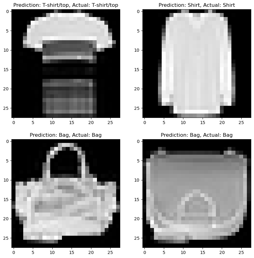
We can see that after 10 epochs, the model could predict the clothing object with 70 % accuracy. Let’s put that to the test.
Visualisation of the Model#
Lets randomly select four examples from the training data and see how the network does.
import numpy as np
import matplotlib.pyplot as plt

rng = np.random.RandomState(42)
samples = rng.randint(0, test_data.data.shape[0], 4)

model.eval()

fig, ax = plt.subplots(2, 2, figsize=(10, 10))
ax = ax.flatten()
for i, sample in enumerate(samples):
    with torch.no_grad():
        pred = model(test_data.data[sample].float().view(1, -1))
        ax[i].imshow(test_data.data[sample], cmap='gray')
        ax[i].set_title(f"Prediction: {classes[pred.argmax(1).item()]}, Actual: {classes[test_data.targets[sample].item()]}")
plt.show()