SciPy Statistical Objects#
The SciPy library has some fantastic functionality for working with statistical objects.
Specifically, here we will look at the scipy.stats.rv_continuous base class (and the discrete sibling, scipy.stats.rv_discrete).
This base class is used to gain access to a range of functionality for different statistical distributions.
We can find a full list of the distributions that can be modelled in the SciPy documentation.
Discrete Distributions#
We will start by looking at the bernoulli distribution.
This can be imported as follows.
from scipy.stats import bernoulli
The Bernoulli distribution has a single parameter, \(p\), so we can create a bernoulli object, which is a super class of the rv_discrete type, that models a fair coin as shown.
p = 0.5

fair_coin = bernoulli(p)
The fair_coin object can be used to simulate a number of coin flips, below we simulate 10 000 and plot the resulting histogram.
import numpy as np
import matplotlib.pyplot as plt

flips = fair_coin.rvs(10_000)

y, x = np.histogram(flips, bins=2, density=True)

fig, ax = plt.subplots()
ax.bar(x[::2], y, width=0.1)
ax.set_xlabel('$k$')
ax.set_ylabel('$P(X=k)$')
ax.set_xticks([0, 1])
ax.set_xticklabels(['Tails', 'Heads'])
plt.show()
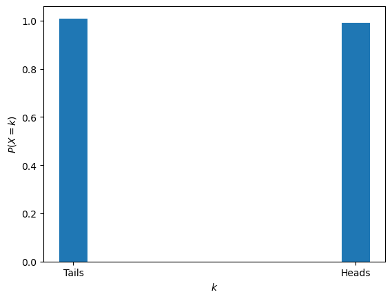
We can see, that over 10 000 observations, the coin appears fair.
The rvs method samples random variables from the distribution.
This method is available for any rv_discrete or rv_continous object.
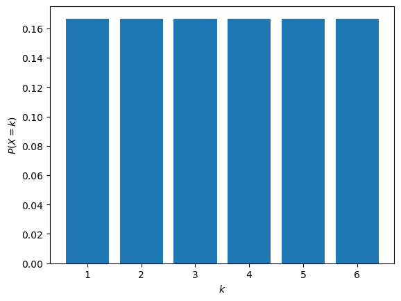
If we wanted to simulate rolling a fair dice, we could use a uniform discrete distribution.
Each side of the fair dice is equally likely.
The uniform discrete distribution in SciPy is called randint.
from scipy.stats import randint

low = 1
high = 7
fair_dice = randint(low, high)
We can plot the PMF of this distribution using the pmf method.
x = np.arange(low, high)

fig, ax = plt.subplots()
ax.bar(x, fair_dice.pmf(x))
ax.set_xlabel('$k$')
ax.set_ylabel('$P(X=k)$')
plt.show()
Continuous Distributions#
The rv_continuous object has many of the same features as the rv_discrete.
So lets look first at the model for a normal distribution.
from scipy.stats import norm

mu = 0
sigma = 1
standard_normal = norm(mu, sigma)

x = np.linspace(-4, 4, 1000)

fig, ax = plt.subplots(1, 2, figsize=(8, 4))
ax[0].plot(x, standard_normal.pdf(x))
ax[0].set_xlabel('$x$')
ax[0].set_ylabel('$P(x)$')
ax[0].set_ylim(0, None)
ax[1].plot(x, standard_normal.cdf(x))
ax[1].set_xlabel('$x$')
ax[1].set_ylabel('$P(X \leq x)$')
ax[1].set_ylim(0, None)
plt.tight_layout()
plt.show()
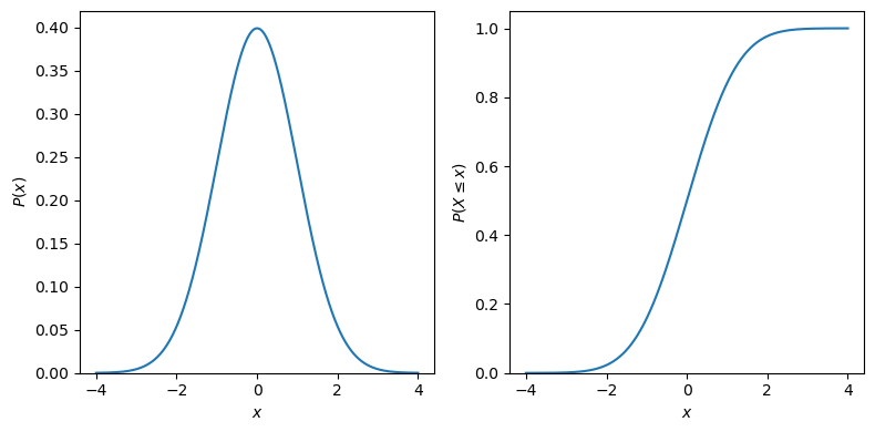
Above, we plot the PDF and CDF for a standard normal distribution. This is a special type of normal distribution where the mean is 0 and the variance (and standard deviation) is 1.
These SciPy objects have a stats method, that can be used to find out the parameters of the distribution.
standard_normal.stats()
(0.0, 1.0)