Markov chain Monte Carlo Sampling

Markov chain Monte Carlo (MCMC) sampling is a powerful and popular approach to likelihood, and posterior sampling. Within the name, there are two concepts that we should try and understand before we look at the implementation of a MCMC algorithm; Markov chains and Monte Carlo.

Monte Carlo

Monte Carlo sampling is an approach used to estimate some numerical result. It is based on the use of random sampling, hoping that we will get an estimate of the true result with enough random samples. A popular example of this you may have seen is using Monte Carlo to estimate π.

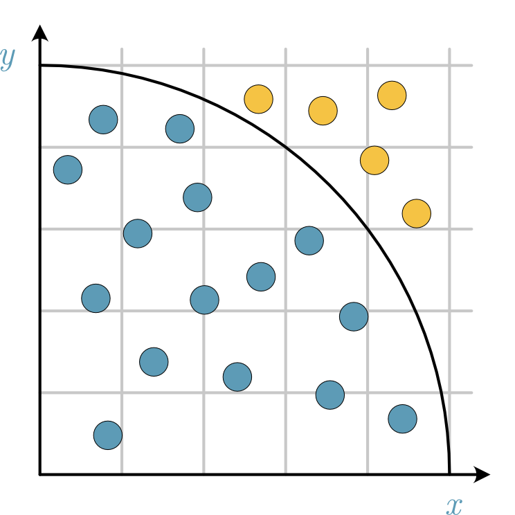
Fig. 32 A diagram showing how the sampling is performed in the Monte Carlo estimation of π, where the stones in the quarter-circle are blue and those outside are yellow.

We can think of this as randomly throwing stones on a square area of 1-by-1 metre. Suppose the stone lands a distance of less than 1 metre from the origin (i.e., the norm of the vector from the stone to the origin is less than 1). In that case, we say it has landed inside the quarter-circle and therefore counts to the integral or area (or the points outside this quarter-cirle are rejected). The area of a quarter-circle is given by,

\[ A_{\textrm{circ}} = \frac{\pi r^2}{4}, \]

where, \(r\) is 1 metre. The area of the 1-by-1 metre square is,

\[ A_{\textrm{squ}} = r^2, \]

and this is approximated by the total number of stones thrown. From computing the ratio of the stones inside the quarter-circle to the total stones thrown, we estimate the following,

\[ \frac{A_{\textrm{circ}}}{A_{\textrm{squ}}} = \frac{\pi r^2}{4} \frac{1}{r^2} = \frac{\pi}{4} \implies \pi = 4 \frac{A_{\textrm{circ}}}{A_{\textrm{squ}}} \]

This can be implemented easily in NumPy code, as shown below, where one million samples were taken/stones were thrown.

import numpy as np
from scipy.stats import uniform

positions = uniform.rvs(loc=0, scale=1, size=(1_000_000, 2))
distances = np.linalg.norm(positions, axis=1)
in_circle = distances[distances < 1]
4 * in_circle.size / distances.size

3.140996

In likelihood sampling, instead of using random samples to estimate an integral, we want to estimate the structure of a probability distribution. However, to make our sampling more efficient, we harness Markov chains.

Markov chains

A Markov chain is a mathematical system, similar in many ways to a random walk. The Markov chain undergoes transitions from one state to another, sampling some (potentially infinite) set of states. Throughout this sampling, the Markov property is followed.

Markov property: the future state depends only on the present state, not the past states’ sequence.

This memorylessness makes Markov chain valuable for application in many areas of science. However, here we will look at how they are used with Monte Carlo rejection to sample a likelihood probability distribution function.

Building an MCMC Algorithm

We will use the first order rate equation data from earlier to look at how this algorithm works. Let’s read this data and set up the model function.

import pandas as pd 
from scipy.stats import norm

data = pd.read_csv('../data/first-order.csv')

D = [norm(data['At'][i], data['At_err'][i]) for i in range(len(data))]

def first_order(t, k, A0):
    """
    A first order rate equation.
    
    :param t: The time to evaluate the rate equation at.
    :param k: The rate constant.
    :param A0: The initial concentration of A.
    
    :return: The concentration of A at time t.
    """
    return A0 * np.exp(-k * t)

It is also necessary to create the likelihood function.

Note

Be aware, that here the likelihood and negative likelihood functions are separate, the reason for this will become clear.

def likelihood(theta):
    """
    The likelihood function for the first order rate equation.
    
    :param theta: The parameters to evaluate the negative likelihood at.
    
    :return: The likelihood at theta.
    """
    return np.sum([d.pdf(first_order(t, theta[0], theta[1])) 
                   for d, t in zip(D, data['t'])])

def negative_likelihood(theta):
    """
    The negative likelihood function for the first order rate equation.
    
    :param theta: The parameters to evaluate the negative likelihood at.
    
    :return: The negative likelihood at theta.
    """
    return -likelihood(theta)

To perform MCMC sampling, we need a place for our algorithm to start from. Using a position close to the maximum likelihood values is common practice. Therefore, below we optimise the negative likelihood to get the parameter values we saw previously.

from scipy.optimize import minimize

res = minimize(negative_likelihood, [0.1, 1])
res.x

array([0.10459843, 7.55723393])

Using these values, we will create ten walkers. These are ten unique Markov chains that we will use in the sampling.

init_chains = norm.rvs(size=(10, 2), random_state=1) * 5e-4 + res.x
init_chains

array([[0.10541061, 7.55692805],
       [0.10433435, 7.55669744],
       [0.10503114, 7.55608316],
       [0.10547084, 7.55685332],
       [0.10475795, 7.55710924],
       [0.10532949, 7.55620385],
       [0.10443723, 7.5570419 ],
       [0.10516532, 7.55668398],
       [0.10451222, 7.556795  ],
       [0.10461954, 7.55752533]])

At this stage we begin the sampling. The MCMC sampling process is shown pictorially in Fig. 33.

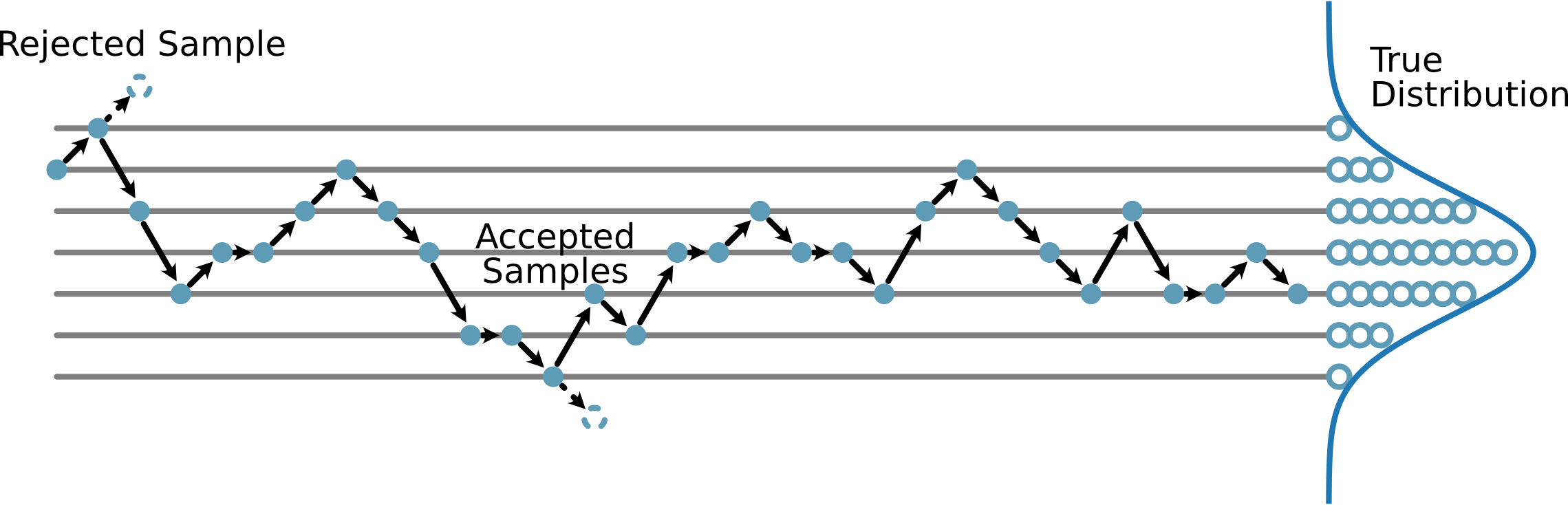
Fig. 33 A pictorial description of how MCMC leads to an estimate of the probability distribution.

The basic idea is to make some pertubation from the previous position and then see how much that has changed the likelihood. If the likelihood has improved, the move is accepted. If the likelihood has decreases, then the move will be accepted if the ratio of the likelihood change is greater than a uniformly sampled random number from 0 to 1. This means that sometimes, we accept moves to lower likelihood, increasing our ability to sample the distribution. If the move is rejected, we store the current value of the parameters. Let’s see that in code.

Note

This algorithm is known as the Metropolis Hastings sampling algorithm [5, 6].

n_samples = 10000
step_std = 5e-3

chains = np.zeros((n_samples, *init_chains.shape))
chains[0] = init_chains
current_likelihood = np.array([likelihood(parameters) for parameters in init_chains])   

for i in range(1, n_samples):
    new_theta = norm(chains[i-1], 
                     np.ones((10, 2)) * step_std).rvs(random_state=i)
    new_likelihood = np.array([likelihood(parameters) 
                               for parameters in new_theta])

    acceptance_ratio = new_likelihood / current_likelihood

    accepted = uniform(loc=0, 
                       scale=1).rvs(size=10, 
                                    random_state=i) < acceptance_ratio
    chains[i] = np.where(accepted[:, np.newaxis], new_theta, chains[i-1])

    current_likelihood = np.array([likelihood(parameters) 
                                   for parameters in chains[i]])   

Note that the step_std value is a hyperparameter for our sampling process that typically requires tuning. After performing all of the sampling, there are two tasks to take care of. The first is reducing autocorrelation and the second is to reshape the samples.

Autocorrelation in Markov Chains

The fact that a Markov chain depends on the previous position can lead to correlation between samples. Consider a particle on a ranomd walk, the position it has reached after some number of steps necessarily affects where it will reach in the next step. It is possible to estimate the autocorrelation time of a Markov chain. Once you know the autocorrelation time, you would typically use every nth sample, where n is that time. This is known as thinning, below, we thin by taking every 10th sample.

flat_chain = chains[::10].reshape(-1, 2)
flat_chain.shape

(10000, 2)

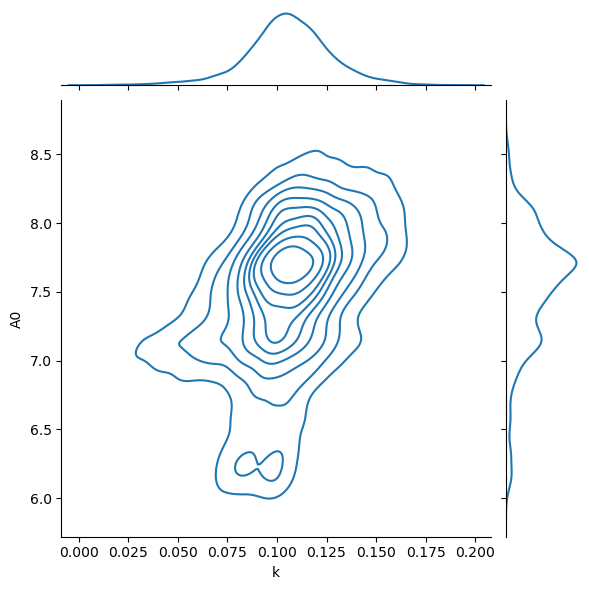
We now have 10 000 independent samples of the two parameters. We can histogram these to get an estimate of the probability density function.

Note

For this figure, we have used seaborn. However, other libraries, such as corner exist for this plotting.

import matplotlib.pyplot as plt
import seaborn as sns

chains_df = pd.DataFrame(flat_chain, columns=['k', 'A0'])
sns.jointplot(data=chains_df, x='k', y='A0', kind='kde')
plt.show()

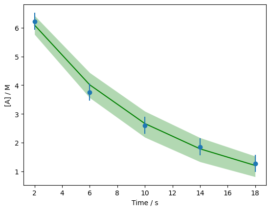
It is possible to then calculate the first order model for all of the values in the flatten chain and plot a range of models that represent the one standard deviation credible interval for the data given the model (the green shaded area).

one_std = first_order(data['t'].values[:, np.newaxis], 
                      flat_chain[:, 0], 
                      flat_chain[:, 1])

fig, ax = plt.subplots()
ax.errorbar(data['t'], data['At'], data['At_err'], fmt='o', zorder=10)
ax.plot(data['t'], np.mean(one_std, axis=1), 'g', zorder=5)
ax.fill_between(data['t'],
                    *np.percentile(one_std, [16, 84], axis=1),
                    alpha=0.3,
                    color='g',
                    lw=0)
ax.set_xlabel('Time / s')
ax.set_ylabel('[A] / M')
plt.show()

Finally, we can compute summary statistics from the flatten chain. However, these should be treated with caution, able we have the whole distribution, not only some single value that describes it.

flat_chain.mean(axis=0), flat_chain.std(axis=0)

(array([0.1057659 , 7.53257799]), array([0.02158326, 0.45250337]))

You may notice the the mean of the flat chain is similar to the maximum likelihood values, but not the same, as the distributions, in particular for \([A]_0\) aren’t completely normally distributed.