k-Means Clustering#
The most straightforward approach to clustering is achieved by creating clusters of particles as close as possible to each other in space. This is essentially what k-means clustering does. From a predefined number of clusters, it uses an Expectation-Maximisation (EM) algorithm to find the optimal position of cluster centres that minimises their Euclidian distance to the data points.
Expectation-Maximisation Algorithm#
The EM algorithm is an iterative optimisation approach popular for finding the best estimates for parameters in statistical models, such as k-means. Generally, this algorithm alternates between two stages:
Expectation: Estimating the model’s parameters and comparing these parameters with the observed data.
Maximisation: Updating the parameters to improve how they describe the observed data.
We will see the EM algorithm appear a few times, so it is nice to consider it in the abstract.
k-Means In Action#
Before discussing the k-mean algorithm, let’s look at what it can do for some of the data transformed into two principal components in the previous section.
import pandas as pd
from sklearn.preprocessing import StandardScaler
from sklearn.decomposition import PCA

data = pd.read_csv('./../data/breast-cancer.csv')
scaled_data = StandardScaler().fit_transform(data[data.columns[1:]])
pca = PCA()
transformed = pca.fit_transform(scaled_data)
pc = pd.DataFrame(transformed, columns=['PC{}'.format(i + 1) for i in range(transformed.shape[1])])
pc['Diagnosis'] = data['Diagnosis']
pc[['PC1', 'PC2']].head()
| PC1 | PC2 | |
|---|---|---|
| 0 | 5.224155 | 3.204428 |
| 1 | 1.728094 | -2.540839 |
| 2 | 3.969757 | -0.550075 |
| 3 | 3.596713 | 6.905070 |
| 4 | 3.151092 | -1.358072 |
As is the case with many of the statistical machine learning approaches, scikit-learn has a useful k-means implementation.
from sklearn.cluster import KMeans

kmeans = KMeans(n_clusters=2)
kmeans.fit(pc[['PC1', 'PC2']])
pc['Cluster'] = kmeans.labels_
The KMeans class follows the standard process of other scikit-learn implementations, with the creation of an object followed by the fitting.
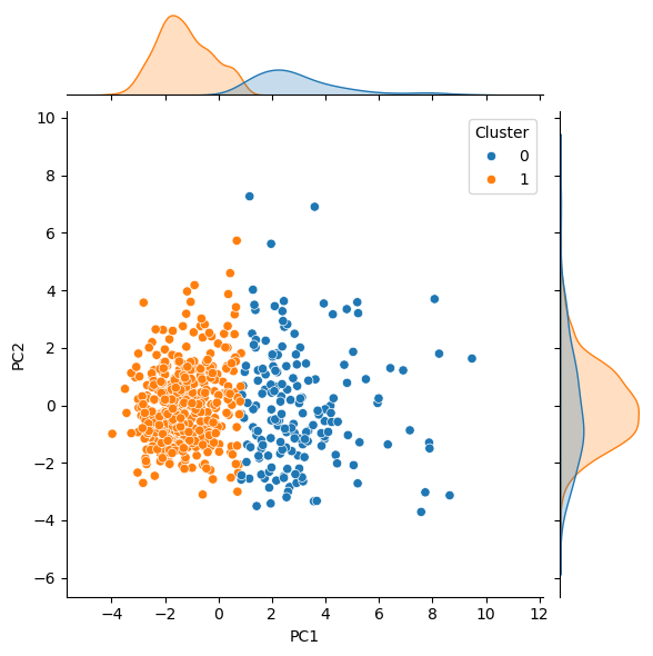
We can visualise these results in the same way we used previously, though this time, the colour indicates the selected cluster for each point.
import matplotlib.pyplot as plt
import seaborn as sns

sns.jointplot(x='PC1', y='PC2', hue='Cluster', data=pc, kind='scatter')
plt.show()
To calculate and assess the accuracy of the PCA followed by clustering, to find the true labels of Benign and Malignant, we map the values to 0 and 1, respectively.
true_labels = pc['Diagnosis'].map({'Malignant': 1, 'Benign': 0})
cluster_labels = pc['Cluster']
Using this, a confusion matrix can be plotted.
from sklearn.metrics import confusion_matrix, ConfusionMatrixDisplay

disp = ConfusionMatrixDisplay(confusion_matrix(true_labels, cluster_labels, normalize='true'),
                              display_labels=['Malignant', 'Benign'])
disp.plot()
plt.show()
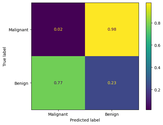
We see that this approach produces a false negative (when the tumour was predicted to be benign but was actually malignent) rate of 1.4%. However, it also had a false positive rate of over 20 %, meaning over 20% of benign tumours were misidentified as malignent. This approach is unlikely to be acceptable for real world use, other then perhaps as an early screening tool to flag for additional testing.
Another scoring method that can be used is an accuracy score.
from sklearn.metrics import accuracy_score

accuracy_score(true_labels, cluster_labels)
0.09666080843585237
This tells us that the accuracy, which is the ratio of correct predictions to total predictions, is 90 %.
As we work through the material, we will look at other metrics for scoring machine learning classification algorithms. But now, let’s look at the k-means algorithm.