Ultranest for Nested Sampling

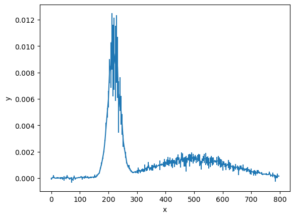
We will look at the following data to investigate nested sampling using the ultranest package.

Note

This signals.csv dataset can be downloaded from this link.

import pandas as pd

data = pd.read_csv('../data/signals.csv')
data.head()

	x	y	yerr
0	0	-5.010978e-05	0.000079
1	4	1.952369e-05	0.000027
2	8	1.091299e-04	0.000130
3	12	3.387135e-09	0.000010
4	16	-6.209843e-06	0.000051

This data is the measurement of some signal \(y\), as a function of \(x\).

import matplotlib.pyplot as plt

fig, ax = plt.subplots()
ax.errorbar(data['x'], data['y'], yerr=data['yerr'])
ax.set_xlabel('x')
ax.set_ylabel('y')
plt.show()

The question we want to answer about this data is if one or two Gaussian signals are present. We can think of this as two models: one for a single signal and a more complex one for two signals. This is the perfect opportunity to use Bayesian model selection.

Before constructing either model, we will create the likelihood function, which will be the same either way but with a different input model.

import numpy as np
from scipy.stats import norm

data_distribution = [norm(loc=loc, scale=scale) for loc, scale in zip(data['y'], data['yerr'])]

def likelihood(params, model):
    """
    A general likelihood function for a model with Gaussian errors.
    
    :param params: The parameters of the model.
    :param model: The model function.
    
    :return: The likelihood of the model given the data.
    """
    model_y = model(data['x'], params)
    return np.sum([d.logpdf(m) for d, m in zip(data_distribution, model_y)])

The next step is to build a simpler model and compute the evidence. We start by creating priors for the mean and standard deviation of the single Gaussian function.

from scipy.stats import uniform, norm

priors_one = [norm(220, 20), 
              uniform(10, 20)]

The mean has a normally distributed prior (\(\mathcal{N}(220, 20)\)) and the standard deviation is uniform (\(\mathcal{U}(10, 20)\)).

The next step is to create a prior transform function. This function converts uniformly distributed random variables to random variables drawn from the priors of interest.

def prior_transform_one(u):
    """
    Transform the uniform random variables `u` to the model parameters.
    
    :param u: Uniform random variables
    
    :return: Model parameters
    """
    return [p.ppf(u_) for p, u_ in zip(priors_one, u)]

Now, we construct the model and create a model-specific likelihood and function to be fed to the sampler.

def model_one(x, params):
    """
    A simpler single Gaussian model.
    
    :param x: The x values
    :param params: The model parameters
    
    :return: The y values
    """
    return norm(loc=params[0], scale=params[1]).pdf(x)

def likelihood_one(params):
    """
    The likelihood function for the simpler model.
    
    :param params: The model parameters
    
    :return: The likelihood
    """
    return likelihood(params, model_one)

This is then passed to the ultranest.ReactiveNestedSampler.

import ultranest

sampler_one = ultranest.ReactiveNestedSampler(['mu1', 'sigma1'], likelihood_one, prior_transform_one)
sampler_one.run(show_status=False)
sampler_one.print_results()

[ultranest] Sampling 400 live points from prior ...

[ultranest] Explored until L=-7e+05  

[ultranest] Likelihood function evaluations: 8424

[ultranest]   logZ = -6.828e+05 +- 0.1387

[ultranest] Effective samples strategy satisfied (ESS = 1594.7, need >400)

[ultranest] Posterior uncertainty strategy is satisfied (KL: 0.46+-0.07 nat, need <0.50 nat)

[ultranest] Evidency uncertainty strategy is satisfied (dlogz=0.14, need <0.5)

[ultranest]   logZ error budget: single: 0.15 bs:0.14 tail:0.01 total:0.14 required:<0.50

[ultranest] done iterating.

logZ = -682752.962 +- 0.212
  single instance: logZ = -682752.962 +- 0.155
  bootstrapped   : logZ = -682752.982 +- 0.211
  tail           : logZ = +- 0.010
insert order U test : converged: True correlation: inf iterations

    mu1                 : 220.664│ ▁  ▁▁▁▁▁▁▁▂▂▃▄▅▇▆▆▇▇▇▅▅▅▅▃▂▂▁▁▁▁▁▁▁▁▁ │221.388    221.035 +- 0.084
    sigma1              : 16.050│ ▁  ▁ ▁▁▁▁▂▂▂▃▄▅▄▇▇▇▇▇▆▅▄▄▂▂▁▁▁▁▁▁▁▁ ▁ │16.542    16.297 +- 0.055

sampler_one.results['logz'], sampler_one.results['logzerr']

(-682752.9617698723, 0.21151762879722505)

We can now do the same process for a more complex two-Gaussian model. Note that we have four priors now instead of two.

priors_two = [norm(220, 20), 
              uniform(10, 20), 
              norm(500, 100),
              uniform(100, 200)]

def prior_transform_two(u):
    """
    Transform the uniform random variables `u` to the model parameters for the more complex model.
    
    :param u: Uniform random variables
    
    :return: Model parameters
    """
    return [p.ppf(u_) for p, u_ in zip(priors_two, u)]

def model_two(x, params):
    """
    A more complex double Gaussian model.
    
    :param x: The x values
    :param params: The model parameters
    
    :return: The y values
    """
    return (norm(loc=params[0], scale=params[1]).pdf(x) + norm(loc=params[2], scale=params[3]).pdf(x)) * 0.5

def likelihood_two(params):
    """
    The likelihood function for the more complex model.
    
    :param params: The model parameters
    
    :return: The likelihood
    """
    return likelihood(params, model_two)

sampler_two = ultranest.ReactiveNestedSampler(['mu1', 'sigma1', 'mu2', 'sigma2'], likelihood_two, prior_transform_two)
sampler_two.run(show_status=False)
sampler_two.print_results()

[ultranest] Sampling 400 live points from prior ...

[ultranest] Explored until L=2e+03  

[ultranest] Likelihood function evaluations: 22323

[ultranest]   logZ = 1564 +- 0.1663

[ultranest] Effective samples strategy satisfied (ESS = 2117.4, need >400)

[ultranest] Posterior uncertainty strategy is satisfied (KL: 0.46+-0.06 nat, need <0.50 nat)

[ultranest] Evidency uncertainty strategy is satisfied (dlogz=0.17, need <0.5)

[ultranest]   logZ error budget: single: 0.22 bs:0.17 tail:0.01 total:0.17 required:<0.50

[ultranest] done iterating.

logZ = 1563.951 +- 0.272
  single instance: logZ = 1563.951 +- 0.222
  bootstrapped   : logZ = 1563.956 +- 0.271
  tail           : logZ = +- 0.010
insert order U test : converged: True correlation: inf iterations

    mu1                 : 219.28│ ▁ ▁▁▁▁▁▁▁▂▂▃▃▅▄▆▆▇▆▇▇▇▆▅▄▃▃▂▂▁▁▁▁▁▁▁▁ │220.44    219.88 +- 0.14
    sigma1              : 19.42 │ ▁▁▁▁▁▁▁▁▁▁▁▂▂▃▄▄▅▆▆▇▆▆▅▅▄▃▃▂▂▁▁▁▁▁▁▁▁ │20.35     19.91 +- 0.11
    mu2                 : 498.35│ ▁▁▁▁▁▁▁▁▂▂▃▃▄▅▅▆▇▇▇▆▇▅▄▃▃▂▁▁▁▁▁▁▁▁ ▁▁ │502.61    500.38 +- 0.49
    sigma2              : 137.79│ ▁▁▁▁▁▁▁▁▁▁▂▂▃▄▄▆▇▆▇▇▇▆▅▅▄▃▃▂▁▁▁▁▁▁▁▁▁ │141.38    139.64 +- 0.41

sampler_two.results['logz'], sampler_two.results['logzerr']

(1563.9514729121147, 0.2715146313839806)

We can now calculate the Bayes factor for these two models.

log_B = sampler_two.results['logz'] - sampler_one.results['logz']
log_B

684316.9132427844

There is decisive evidence for the more complex model. Therefore, we would be able to continue our analysis by considering the signal shown by the two Gaussians.