Support Vector Machines#
An alternative classification to logistic regression is support vector machines. The support vector machine (SVM) aims to find the best linear hyperplane that separates the classes in feature space. This is achieved by maximising the so-called margin, which is the distance between the hyperplane and the nearest data points from each class. These data points are the support vectors.
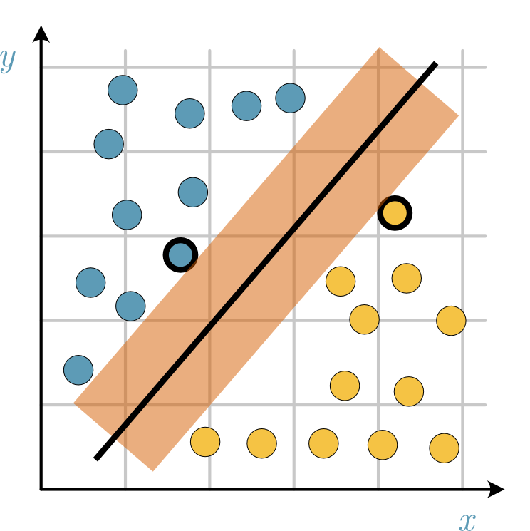
Fig. 27 The margin (represented with the red shaded area) describes the region that separates the yellow and blue support vectors (thick black edge).#
Similar to logistic regression, the hyperplane that an SVM tries to find has the equation,
The two hyperplanes that describe the edges of the margin can be written as
where the items are of class 1, and
for class -1.
The distance between these two hyperplanes is \(\frac{2}{|w|}\), so by minimising \(|\mathbf{w}|\), the maximise this distance.
However, keeping data points on their correct side of the margin is also necessary, which is achieved with an appropriate constraint.
Soft Margin#
It may be impossible to find a hyperplane that completely separates the classes. For example, consider the data from the toy example for logistic regression.
import pandas as pd
import matplotlib.pyplot as plt
import seaborn as sns

data = pd.read_csv("../data/toy.csv")

fix, ax = plt.subplots()
sns.scatterplot(x='x', y='y', data=data, hue='label', ax=ax)
plt.show()
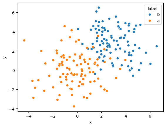
It is clear that due to the overlap, no hyperplane is possible. SVMs handle this by including what is known as a soft margin. The soft margin introduces some allowance for misclassification of data points. This leads the loss function to be the hinge loss,
where \(C\) is the hyperparameter that controls the trade-off between maximising the margin and minimising misclassification.
Putting It Into Practice#
Let’s see if we can develop a support vector machine to classify our toy data. Once again, we will split the data in the same way as previously to enable comparison and create separate objects for the training dataset.
from sklearn.model_selection import train_test_split

data['encoded_label'] = [1 if i == 'b' else 0 for i in data['label'].values]
train, test = train_test_split(data, test_size=0.2, random_state=0)
X = train[['x', 'y']].values
y = train['encoded_label'].values
Again, we generate our initial weights and bias.
import numpy as np

rng = np.random.default_rng(1)
weights = rng.standard_normal(2)
bias = rng.standard_normal(1)
weights, bias
(array([0.34558419, 0.82161814]), array([0.33043708]))
The next step is to define the loss function, learning rate and \(C\). Again, we use JAX here to help our gradient descent algorithm.
import jax.numpy as jnp
from jax import grad

C = 0.1
learning_rate = 0.001

def loss_function(weights, bias):
    prediction = y * (jnp.dot(X, weights) + bias)
    stack = jnp.hstack([jnp.zeros_like(y), 1 - prediction])
    soft_margin = C * jnp.mean(jnp.max(stack, axis=0))
    return 0.5 * jnp.linalg.norm(weights) ** 2 + soft_margin

first_order = grad(loss_function)
We now run 2000 iterations of the gradient descent algorithm.
result = grad(loss_function)(weights, bias)

for i in range(2000):
    weights = weights - learning_rate * result[:-1]
    bias = bias - learning_rate * result[-1]
    result = grad(loss_function)(weights, bias)
We compute the accuracy score against the training and test data as before.
from sklearn.metrics import accuracy_score

z = np.dot(train[['x', 'y']], weights) + bias
f = np.sign(z)
prediction = np.array(['nd'] * len(z))
prediction[np.where(f > 0)] = 'b'
prediction[np.where(f < 0)] = 'a'
train['prediction'] = prediction
z
accuracy_score(train['label'], train['prediction'])
0.86875
z = np.dot(test[['x', 'y']], weights) + bias
f = np.sign(z)
prediction = np.array(['x'] * len(f))
prediction[np.where(f > 0)] = 'b'
prediction[np.where(f < 0)] = 'a'
test['prediction'] = prediction

accuracy_score(test['label'], test['prediction'])
0.875
This gives similar, but slightly different, values to the logistic regression. This is expected, as we are optimising different functions to enable the discrimination.
Thus far, both methods are limited to data with linear discrimination. Let’s look at a tool employed by support vector machines to help in this area.