Neural Network Policies#
Neural networks are highly effective for training reinforcement learning algorithms.
Similar to other neural network examples, it can be hard to interpret the optimised network.
Let’s try to build a network to train for this LunarLander-v3.
Our policy network will be a simple three-linear layer network.
import torch.nn as nn
import torch.nn.functional as F

class QNetwork(nn.Module):
    """
    A simple feedforward neural network with 2 hidden layers.

    :param obs_dim: The dimension of the input obs.
    :param action_dim: The dimension of the output action.
    """
    def __init__(self, obs_dim, action_dim):
        super(QNetwork, self).__init__()
        self.fc1 = nn.Linear(obs_dim, 128)
        self.fc2 = nn.Linear(128, 128)
        self.fc3 = nn.Linear(128, action_dim)

    def forward(self, x):
        """
        Forward pass of the network.

        :param x: The input obs.
        :return: The output action.
        """
        x = F.relu(self.fc1(x))
        x = F.relu(self.fc2(x))
        return self.fc3(x)
However, the broader training strategy will involve using a deep Q-network. This approach uses a Replay Buffer, which reduces the correlation between episodes while enabling the reuse of past experiences. For more on this structure, there is a good Stack Exchange answer on the subject. We construct below the Replay Buffer class.
import random
from collections import deque

class ReplayBuffer:
    """
    A simple replay buffer for storing experiences.

    :param capacity: The maximum capacity of the buffer.
    """
    def __init__(self, capacity):
        self.buffer = deque(maxlen=capacity)

    def push(self, obs, action, reward, next_obs, done):
        """
        Push an experience to the buffer.

        :param obs: The current obs.
        :param action: The action taken.
        :param reward: The reward received.
        :param next_obs: The next obs.
        :param done: Whether the episode is done.
        """
        self.buffer.append((obs, action, reward, next_obs, done))

    def sample(self, batch_size):
        """
        Sample a batch of experiences from the buffer.

        :param batch_size: The size of the batch.
        :return: The batch of experiences.
        """
        return random.sample(self.buffer, batch_size)

    def __len__(self):
        """
        :return: The length of the buffer.
        """
        return len(self.buffer)
The final stage is to build the training loop. This is where the Q-learning component comes in. We can think of Q-learning as a table that stores the best learning actions, where each cell holds a Q-value and estimates how good that action is for a given state of the environment. The Q-values are then updated iteratively using the Bellman equation,
where \(s\) and \(s'\) are the current and next observations, \(a\) and \(a'\) are the current and next actions, \(r\) is the reward received for the next action, \(\alpha\) is the learning rate, and $\gamma is the discount factor, which controls how much future rewards matter.
Here, we use a deep Q-network, so the neural network estimates them instead of explicitly computing the Q-values.
To enable this, we create two networks, the policy_net and the target_net, which provide the Qvalues for the next observation.
To add some randomness to the network, we have a Monte Carlo step utilised in a simulated annealing fashion.
This means the likelihood that the Monte Carlo (randomly selected) policy is used decreases as the training progresses.
The EPSILON_DECAY hyperparameter controls the amount that this decreases.
import numpy as np
import torch
import torch.optim as optim

GAMMA = 0.99
LEARNING_RATE = 1e-3
BATCH_SIZE = 64
BUFFER_SIZE = 10000
EPSILON_DECAY = 0.995
MIN_EPSILON = 0.01
TARGET_UPDATE = 10

def train(env, episodes=1000):
    obs_dim = env.observation_space.shape[0]
    action_dim = env.action_space.n

    policy_net = QNetwork(obs_dim, action_dim)
    target_net = QNetwork(obs_dim, action_dim)
    target_net.load_state_dict(policy_net.state_dict())
    target_net.eval()

    optimizer = optim.Adam(policy_net.parameters(), lr=LEARNING_RATE)
    replay_buffer = ReplayBuffer(BUFFER_SIZE)
    epsilon = np.ones(episodes)
    total_reward = np.zeros(episodes)

    for episode in range(episodes):
        obs, _ = env.reset()
        obs = torch.tensor(obs, dtype=torch.float32).unsqueeze(0)
        done = False

        while not done:
            if random.random() < epsilon[episode]:
                action = env.action_space.sample()
            else:
                with torch.no_grad():
                    action = policy_net(obs).argmax().item()

            next_obs, reward, terminated, truncated, _ = env.step(action)
            done = terminated or truncated
            next_obs = torch.tensor(next_obs, dtype=torch.float32).unsqueeze(0)
            replay_buffer.push(obs, action, reward, next_obs, done)

            obs = next_obs
            total_reward[episode] += reward

            if len(replay_buffer) >= BATCH_SIZE:
                batch = replay_buffer.sample(BATCH_SIZE)
                obss, actions, rewards, next_obss, dones = zip(*batch)

                obss = torch.cat(obss)
                actions = torch.tensor(actions, dtype=torch.int64).unsqueeze(1)
                rewards = torch.tensor(rewards, dtype=torch.float32).unsqueeze(1)
                next_obss = torch.cat(next_obss)
                dones = torch.tensor(dones, dtype=torch.float32).unsqueeze(1)

                q_values = policy_net(obss).gather(1, actions)
                next_q_values = target_net(next_obss).max(1, keepdim=True)[0]
                target_q_values = rewards + GAMMA * next_q_values * (1 - dones)

                loss = F.mse_loss(q_values, target_q_values.detach())
                optimizer.zero_grad()
                loss.backward()
                optimizer.step()

        if episode % TARGET_UPDATE == 0:
            target_net.load_state_dict(policy_net.state_dict())

        if episode < episodes - 1:
            epsilon[episode+1] = max(MIN_EPSILON, epsilon[episode] * EPSILON_DECAY)

    return policy_net, total_reward, epsilon
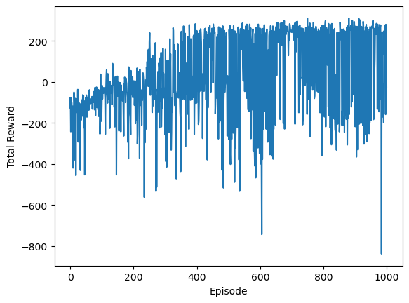
We can now train the network to over 1000 episodes.
import gymnasium as gym

env = gym.make('LunarLander-v3', render_mode='rgb_array')
trained_policy, nn_training_rewards, epsilon = train(env)
/usr/share/miniconda/envs/special-topics/lib/python3.11/site-packages/pygame/pkgdata.py:25: UserWarning: pkg_resources is deprecated as an API. See https://setuptools.pypa.io/en/latest/pkg_resources.html. The pkg_resources package is slated for removal as early as 2025-11-30. Refrain from using this package or pin to Setuptools<81.
  from pkg_resources import resource_stream, resource_exists
And plot the reward trend as a function of the episode. Note the slight upward trend over the training time.
import matplotlib.pyplot as plt

fig, ax = plt.subplots()

ax.plot(nn_training_rewards)
ax.set_xlabel('Episode')
ax.set_ylabel('Total Reward')
plt.show()
We can now use this trained policy over another 500 random episodes to see how it compares to the modulo and logical policies.
nn_rewards = np.zeros((500))
render = None
for repeat in range(nn_rewards.shape[0]):
    current_rewards = 0
    obs = env.reset()[0]
    current_render = []
    for step in range(env.spec.max_episode_steps):
        action = trained_policy(torch.tensor(obs, dtype=torch.float32).unsqueeze(0)).argmax().item()
        obs, reward, terminated, truncated, info = env.step(action)
        current_rewards += reward
        current_render.append(env.render())
        if terminated:
            break
    if current_rewards > nn_rewards.max():
        render = current_render
    nn_rewards[repeat] = current_rewards

    env.close()
total_rewards = np.loadtxt('total_rewards.txt')

fig, ax = plt.subplots()

ax.hist(total_rewards[0], label='Modulo Policy', density=True)
ax.hist(total_rewards[1], label='Logical Policy', density=True)
ax.hist(nn_rewards, label='Neural Network Policy', density=True)
ax.legend()
ax.set_xlabel('Reward')
ax.set_ylabel('p(Reward)')
plt.show()
---------------------------------------------------------------------------
FileNotFoundError                         Traceback (most recent call last)
Cell In[7], line 1
----> 1 total_rewards = np.loadtxt('total_rewards.txt')
      3 fig, ax = plt.subplots()
      5 ax.hist(total_rewards[0], label='Modulo Policy', density=True)

File /usr/share/miniconda/envs/special-topics/lib/python3.11/site-packages/numpy/lib/npyio.py:1373, in loadtxt(fname, dtype, comments, delimiter, converters, skiprows, usecols, unpack, ndmin, encoding, max_rows, quotechar, like)
   1370 if isinstance(delimiter, bytes):
   1371     delimiter = delimiter.decode('latin1')
-> 1373 arr = _read(fname, dtype=dtype, comment=comment, delimiter=delimiter,
   1374             converters=converters, skiplines=skiprows, usecols=usecols,
   1375             unpack=unpack, ndmin=ndmin, encoding=encoding,
   1376             max_rows=max_rows, quote=quotechar)
   1378 return arr

File /usr/share/miniconda/envs/special-topics/lib/python3.11/site-packages/numpy/lib/npyio.py:992, in _read(fname, delimiter, comment, quote, imaginary_unit, usecols, skiplines, max_rows, converters, ndmin, unpack, dtype, encoding)
    990     fname = os.fspath(fname)
    991 if isinstance(fname, str):
--> 992     fh = np.lib._datasource.open(fname, 'rt', encoding=encoding)
    993     if encoding is None:
    994         encoding = getattr(fh, 'encoding', 'latin1')

File /usr/share/miniconda/envs/special-topics/lib/python3.11/site-packages/numpy/lib/_datasource.py:193, in open(path, mode, destpath, encoding, newline)
    156 """
    157 Open `path` with `mode` and return the file object.
    158
   (...)    189
    190 """
    192 ds = DataSource(destpath)
--> 193 return ds.open(path, mode, encoding=encoding, newline=newline)

File /usr/share/miniconda/envs/special-topics/lib/python3.11/site-packages/numpy/lib/_datasource.py:533, in DataSource.open(self, path, mode, encoding, newline)
    530     return _file_openers[ext](found, mode=mode,
    531                               encoding=encoding, newline=newline)
    532 else:
--> 533     raise FileNotFoundError(f"{path} not found.")

FileNotFoundError: total_rewards.txt not found.
We can see that with no hyperparameter optimisation, the neural network policy is, on average, outperforming the other two approaches.