k-Means Algorithm

The EM algorithm for k-means has the following procedure:

1. Guess some initial cluster centres.

2. Repeat the following until convergence is reached:

   1. E-step: Assign points to the nearest cluster centre.

   2. M-step: Update the cluster centres with the mean position.

The E-step updates our expectation of which cluster each point belongs to, while the M-step maximises some fitness function that defines the cluster centre locations. Each repetition of the E-M loop will always result in a better estimate of the cluster characteristics.

Let’s write some code to perform this algorithm ourselves. First, we need some data to cluster; for this, we will use the scikit-learn method to produce random blobs of data.

import numpy as np
import matplotlib.pyplot as plt

X = np.loadtxt('../data/kmeans.txt')
fig, ax = plt.subplots(figsize=(6, 4))
ax.plot(X[:, 0], X[:, 1], '.')
plt.show()

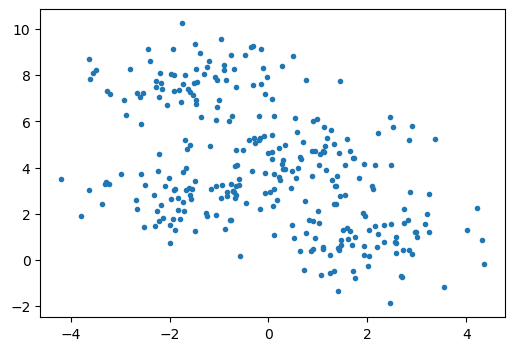
We will try to identify four clusters in this data. Therefore, we set the following.

n_clusters = 4

As a starting position, let’s select four of the points randomly.

import numpy as np

i = np.random.randint(0, X.shape[0], size=4)
centres = X[i]

Our initial guess is shown below with orange squares.

fig, ax = plt.subplots(figsize=(6, 4))
ax.plot(X[:, 0], X[:, 1], '.')
ax.plot(centres[:, 0], centres[:, 1], 's')
plt.show()

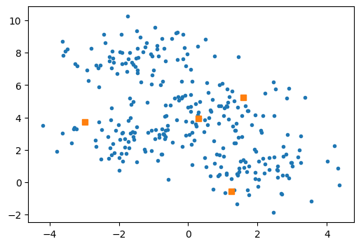
It is clear that they do not represent the arithmetic mean of any data. The second step (the first of the E-M loop) assigns all the points to their nearest cluster centre. This can be achieved very efficiently by using NumPy and array broadcasting. First, we compute the vector from each of the data, X, to each current cluster centre.

vectors = X[:, np.newaxis] - centres
vectors.shape

(300, 4, 2)

Notice that the shape of this array is (number_of_data, number_of_clusters, dimensions). The magnitude of the vector can describe the distance from the data to the current centres; we want the magnitude along the dimensions axis of the array (the final axis, hence -1).

magnitudes = np.linalg.norm(vectors, axis=-1)
magnitudes.shape

(300, 4)

We now have the magnitude of the vector from each data point to each cluster centre. We want to know which centre each datapoint is closest to; we can use the argmin() method of the NumPy array. This returns the index of the minimum value (the method min() will return the actual value, but we aren’t interested in this). The argmin() method should only be run on the number of clusters axis to end up with an array of 300 indices.

labels = magnitudes.argmin(axis=1)
print(labels)

[1 3 2 3 1 0 1 2 3 3 1 3 2 3 0 1 2 0 1 1 0 0 1 1 1 1 0 1 1 1 3 3 2 3 3 3 3
 3 1 0 1 1 3 2 1 1 3 1 3 0 1 0 3 0 1 1 2 1 3 1 3 1 3 1 1 1 3 0 3 1 2 1 3 1
 1 3 1 2 0 3 0 1 1 0 3 2 0 1 3 3 1 0 3 1 1 1 1 0 3 1 3 0 3 0 2 0 0 2 3 2 1
 1 0 3 0 2 3 1 1 1 1 0 1 0 1 0 0 1 1 1 3 1 1 0 3 1 1 3 1 3 3 1 1 1 2 1 3 1
 3 3 3 1 1 1 0 1 3 1 0 2 3 1 1 1 1 1 1 1 1 1 1 3 0 2 1 3 0 0 1 1 0 2 1 1 1
 2 2 1 0 3 1 1 1 1 1 1 1 2 1 3 1 1 0 1 1 1 1 3 2 3 2 1 1 2 3 1 1 0 0 1 3 0
 0 1 0 1 1 3 3 2 1 3 1 1 1 1 0 1 3 1 0 1 0 3 3 3 3 1 1 1 2 1 0 1 1 1 1 0 0
 3 1 1 1 0 3 1 2 3 2 0 0 1 1 2 0 0 1 2 3 3 0 0 2 0 0 0 3 1 3 1 0 0 3 3 3 1
 0 1 2 1]

This array, labels, assigns each data point to the closest cluster centres, completing the E-step in the E-M loop. Now, we need to update the cluster centres with the new arithmetic mean of the assigned data. The data can be split into groups using logical slicing i.e., to get all values with the label 0.

X[labels == 0]

array([[ 4.35918422, -0.16235216],
       [ 1.05505217, -0.64710744],
       [ 2.91209813,  0.24663807],
       [ 3.15492712,  1.55292739],
       [ 1.59167155,  1.37914513],
       [ 1.45895348,  0.84509636],
       [ 1.40285894,  0.50671028],
       [ 1.94472686,  1.91783637],
       [ 2.7216506 ,  0.43694387],
       [ 1.45795145,  0.65974193],
       [ 2.57915855,  0.98608575],
       [ 2.19722068,  0.57833524],
       [ 0.72100905, -0.44905385],
       [ 1.51240605,  1.31371371],
       [ 2.57854418,  0.72611733],
       [ 1.59973502,  0.91514282],
       [ 2.96544643,  1.21488188],
       [ 1.41164912, -1.32573949],
       [ 2.5763324 ,  0.32187569],
       [ 2.34161121,  1.50650749],
       [ 2.69539905, -0.71929238],
       [ 1.25185786,  0.20811388],
       [ 1.68608568,  0.65828448],
       [ 1.42717996,  0.41663654],
       [ 0.86640826,  0.39084731],
       [ 2.03824711,  1.2768154 ],
       [ 1.4178305 ,  0.50039185],
       [ 2.68049897, -0.704394  ],
       [ 1.24190326, -0.56876067],
       [ 1.74438135,  0.99506383],
       [ 1.09932252,  0.55168188],
       [ 2.74508569,  2.19950989],
       [ 2.48152625,  1.57457169],
       [ 3.00468833,  0.9852149 ],
       [ 2.74680627,  1.5924128 ],
       [ 1.74625455, -0.77834015],
       [ 1.93710348,  0.21748546],
       [ 3.54975207, -1.17232137],
       [ 2.84159548,  0.43124456],
       [ 2.0309414 ,  0.15963275],
       [ 1.32967014, -0.4857003 ],
       [ 1.92238694,  0.59987278],
       [ 3.24329731,  1.21460627],
       [ 4.31457647,  0.85540651],
       [ 1.11082127,  0.48761397],
       [ 2.0159847 , -0.27042984],
       [ 2.21177406,  1.1298447 ],
       [ 0.90779887,  0.45984362],
       [ 2.15299249,  1.48061734],
       [ 0.63120661,  0.40434378],
       [ 4.21850347,  2.23419161],
       [ 1.70127361, -0.47728763],
       [ 3.20759909,  1.97728225],
       [ 2.97612635,  1.21639131],
       [ 2.5490093 ,  0.78155972],
       [ 2.33519212,  0.79951327],
       [ 4.01117983,  1.28775698],
       [ 2.45431387, -1.8749291 ],
       [ 1.65581849,  1.26771955],
       [ 2.82705807,  1.72116781]])

Above are all the datapoints associated with the first cluster centre, and the mean (along the datapoint axis can be found as).

X[labels == 0].mean(axis=0)

array([2.19252731, 0.59246049])

And it is possible to perform this for all four clusters with simple list comprehension.

new_centres = np.array([X[labels == i].mean(axis=0) for i in range(n_clusters)])

The new centres can be visualised below (this time with triangles).

fig, ax = plt.subplots(figsize=(6, 4))
ax.plot(X[:, 0], X[:, 1], '.')
ax.plot(centres[:, 0], centres[:, 1], 's')
ax.plot(new_centres[:, 0], new_centres[:, 1], '^')
plt.show()

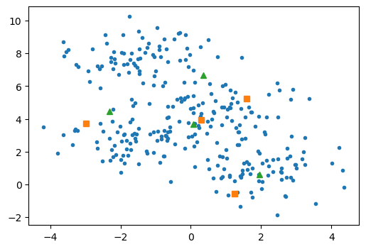
Finally, we overwrite the centres object to update the centres.

centres = new_centres

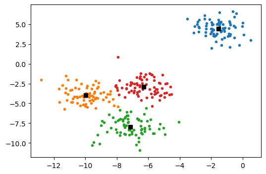
This process should be completed until the centres do not change so we can use an iterative approach. See the code cell below, which loops over this process until there is no change in the centres.

from sklearn.datasets import make_blobs
import numpy as np

X, y_true = make_blobs(n_samples=300, centers=4, cluster_std=1, random_state=1)
n_clusters = 4
i = np.random.randint(0, X.shape[0], size=n_clusters)
centres = X[i]
diff = np.inf
while np.sum(diff) > 0.00000001:
    vectors = X[:, np.newaxis] - centres
    magnitudes = np.linalg.norm(vectors, axis=-1)
    labels = magnitudes.argmin(axis=1)
    new_centres = np.array([X[labels == i].mean(axis=0) for i in range(n_clusters)])
    diff = np.abs(centres - new_centres)
    centres = new_centres

We show the results below, with the different clusters identified by colour and the cluster centres marked with a black square.

from sklearn.cluster import KMeans

fig, ax = plt.subplots(figsize=(6, 4))
for i in range(n_clusters):
    ax.plot(X[labels == i][:, 0], X[labels == i][:, 1], '.')
ax.plot(centres[:, 0], centres[:, 1], 'ks')
plt.show()

There are some important issues that one should be aware of in using the simple E-M algorithm discussed above:

• The optimal result may never be achieved globally. As with all optimisation routines, although the result is improving, it may not be moving to the globally optimal solution.

• k-means is limited to linear cluster boundaries. The fact that k-means finds samples as close as possible in cartesian space means that the clustering cannot have more complex geometries.

• k-means can be slow for a large number of samples. Each iteration must access every point in the dataset (and in our implementation, it accesses each point n_clusters number of times)!

• The number of clusters must be selected beforehand. We must have some a priori knowledge about our dataset to apply a k-means clustering effectively.

This final point is a common concern in k-means clustering and other clustering algorithms. Therefore, let’s look at a popular tool used to find the “correct” number of clusters.