Datasets#
Let’s look at the openly available datasets we will use in detail. Many of these will be used for both unsupervised and supervised approaches.
Abalone Dataset#
This data was sourced from the UC Irvine Machine Learning Repository. The file has been modified to include the names of the features and can be downloaded here.
Let’s have a look at this dataset.
import pandas as pd

data = pd.read_csv('./../data/abalone.csv')
data
| Sex | Length/mm | Diameter/mm | Height/mm | Whole Weight/g | Shucked Weight/g | Viscera Weight/g | Shell Weight/g | Rings | |
|---|---|---|---|---|---|---|---|---|---|
| 0 | M | 0.455 | 0.365 | 0.095 | 0.5140 | 0.2245 | 0.1010 | 0.1500 | 15 |
| 1 | M | 0.350 | 0.265 | 0.090 | 0.2255 | 0.0995 | 0.0485 | 0.0700 | 7 |
| 2 | F | 0.530 | 0.420 | 0.135 | 0.6770 | 0.2565 | 0.1415 | 0.2100 | 9 |
| 3 | M | 0.440 | 0.365 | 0.125 | 0.5160 | 0.2155 | 0.1140 | 0.1550 | 10 |
| 4 | I | 0.330 | 0.255 | 0.080 | 0.2050 | 0.0895 | 0.0395 | 0.0550 | 7 |
| ... | ... | ... | ... | ... | ... | ... | ... | ... | ... |
| 4172 | F | 0.565 | 0.450 | 0.165 | 0.8870 | 0.3700 | 0.2390 | 0.2490 | 11 |
| 4173 | M | 0.590 | 0.440 | 0.135 | 0.9660 | 0.4390 | 0.2145 | 0.2605 | 10 |
| 4174 | M | 0.600 | 0.475 | 0.205 | 1.1760 | 0.5255 | 0.2875 | 0.3080 | 9 |
| 4175 | F | 0.625 | 0.485 | 0.150 | 1.0945 | 0.5310 | 0.2610 | 0.2960 | 10 |
| 4176 | M | 0.710 | 0.555 | 0.195 | 1.9485 | 0.9455 | 0.3765 | 0.4950 | 12 |
4177 rows × 9 columns
We can see that the data has 4177 entries, each with nine features. These nine features describe the size of the abalone samples (length, diameter, weight, etc.) and the number of rings in their shells. This final feature is a descriptor of the age of the abalone. The number of rings is not straightforward to measure, so estimating the age from these other parameters is desirable.
Before we continue, we must check for any missing data. Missing data would typically be stored as a null value.
pd.isnull(data).sum()
Sex                 0
Length/mm           0
Diameter/mm         0
Height/mm           0
Whole Weight/g      0
Shucked Weight/g    0
Viscera Weight/g    0
Shell Weight/g      0
Rings               0
dtype: int64
We can see no features with missing data (i.e., no null values). If null values were present, depending on the algorithm being used, it may be necessary to remove these data points.
In addition to checking for missing data, we should also consider the nature of some of the data present.
For example, the sex data is not numerical, either male or female.
This data is referred to as categorical, as it has categories.
Similar to missing data, this may not be compatible with the algorithms we apply.
Breast Cancer#
Another dataset that we will look at is the Wisconson Breast Cancer dataset, also sourced from the UC Irvine Machine Learning Repository. This dataset contains information about the size, shape, and texture of breast cancer tumours and has been tagged with information about whether the tumour was found to be benign (not harmful in effect) or malignant (harmful). This dataset has been reduced to suit the pedagogical purposes of this work more and can be downloaded here. Let’s look at the dataset.
data = pd.read_csv('./../data/breast-cancer.csv')
data
| Diagnosis | Radius | Texture | Perimeter | Area | Smoothness | Compactness | Concavity | Concave Points | Symmetry | Fractal Dimension | |
|---|---|---|---|---|---|---|---|---|---|---|---|
| 0 | Malignant | 17.99 | 10.38 | 122.80 | 1001.0 | 0.11840 | 0.27760 | 0.30010 | 0.14710 | 0.2419 | 0.07871 |
| 1 | Malignant | 20.57 | 17.77 | 132.90 | 1326.0 | 0.08474 | 0.07864 | 0.08690 | 0.07017 | 0.1812 | 0.05667 |
| 2 | Malignant | 19.69 | 21.25 | 130.00 | 1203.0 | 0.10960 | 0.15990 | 0.19740 | 0.12790 | 0.2069 | 0.05999 |
| 3 | Malignant | 11.42 | 20.38 | 77.58 | 386.1 | 0.14250 | 0.28390 | 0.24140 | 0.10520 | 0.2597 | 0.09744 |
| 4 | Malignant | 20.29 | 14.34 | 135.10 | 1297.0 | 0.10030 | 0.13280 | 0.19800 | 0.10430 | 0.1809 | 0.05883 |
| ... | ... | ... | ... | ... | ... | ... | ... | ... | ... | ... | ... |
| 564 | Malignant | 21.56 | 22.39 | 142.00 | 1479.0 | 0.11100 | 0.11590 | 0.24390 | 0.13890 | 0.1726 | 0.05623 |
| 565 | Malignant | 20.13 | 28.25 | 131.20 | 1261.0 | 0.09780 | 0.10340 | 0.14400 | 0.09791 | 0.1752 | 0.05533 |
| 566 | Malignant | 16.60 | 28.08 | 108.30 | 858.1 | 0.08455 | 0.10230 | 0.09251 | 0.05302 | 0.1590 | 0.05648 |
| 567 | Malignant | 20.60 | 29.33 | 140.10 | 1265.0 | 0.11780 | 0.27700 | 0.35140 | 0.15200 | 0.2397 | 0.07016 |
| 568 | Benign | 7.76 | 24.54 | 47.92 | 181.0 | 0.05263 | 0.04362 | 0.00000 | 0.00000 | 0.1587 | 0.05884 |
569 rows × 11 columns
Similar to the abalone dataset, the null values have been stripped from the data.
pd.isnull(data).sum()
Diagnosis            0
Radius               0
Texture              0
Perimeter            0
Area                 0
Smoothness           0
Compactness          0
Concavity            0
Concave Points       0
Symmetry             0
Fractal Dimension    0
dtype: int64
Handwritten Digits Dataset#
A popular dataset for looking at machine learning algorithms is the MNIST handwritten digits dataset. This data contains a series of images of digits that have been handwritten. Let’s load the data in and have a look at the structure.
data = pd.read_csv('./../data/mnist.csv')

data
| pixel1 | pixel2 | pixel3 | pixel4 | pixel5 | pixel6 | pixel7 | pixel8 | pixel9 | pixel10 | ... | pixel776 | pixel777 | pixel778 | pixel779 | pixel780 | pixel781 | pixel782 | pixel783 | pixel784 | label | |
|---|---|---|---|---|---|---|---|---|---|---|---|---|---|---|---|---|---|---|---|---|---|
| 0 | 0 | 0 | 0 | 0 | 0 | 0 | 0 | 0 | 0 | 0 | ... | 0 | 0 | 0 | 0 | 0 | 0 | 0 | 0 | 0 | 5 |
| 1 | 0 | 0 | 0 | 0 | 0 | 0 | 0 | 0 | 0 | 0 | ... | 0 | 0 | 0 | 0 | 0 | 0 | 0 | 0 | 0 | 0 |
| 2 | 0 | 0 | 0 | 0 | 0 | 0 | 0 | 0 | 0 | 0 | ... | 0 | 0 | 0 | 0 | 0 | 0 | 0 | 0 | 0 | 4 |
| 3 | 0 | 0 | 0 | 0 | 0 | 0 | 0 | 0 | 0 | 0 | ... | 0 | 0 | 0 | 0 | 0 | 0 | 0 | 0 | 0 | 1 |
| 4 | 0 | 0 | 0 | 0 | 0 | 0 | 0 | 0 | 0 | 0 | ... | 0 | 0 | 0 | 0 | 0 | 0 | 0 | 0 | 0 | 9 |
| ... | ... | ... | ... | ... | ... | ... | ... | ... | ... | ... | ... | ... | ... | ... | ... | ... | ... | ... | ... | ... | ... |
| 19995 | 0 | 0 | 0 | 0 | 0 | 0 | 0 | 0 | 0 | 0 | ... | 0 | 0 | 0 | 0 | 0 | 0 | 0 | 0 | 0 | 9 |
| 19996 | 0 | 0 | 0 | 0 | 0 | 0 | 0 | 0 | 0 | 0 | ... | 0 | 0 | 0 | 0 | 0 | 0 | 0 | 0 | 0 | 5 |
| 19997 | 0 | 0 | 0 | 0 | 0 | 0 | 0 | 0 | 0 | 0 | ... | 0 | 0 | 0 | 0 | 0 | 0 | 0 | 0 | 0 | 1 |
| 19998 | 0 | 0 | 0 | 0 | 0 | 0 | 0 | 0 | 0 | 0 | ... | 0 | 0 | 0 | 0 | 0 | 0 | 0 | 0 | 0 | 4 |
| 19999 | 0 | 0 | 0 | 0 | 0 | 0 | 0 | 0 | 0 | 0 | ... | 0 | 0 | 0 | 0 | 0 | 0 | 0 | 0 | 0 | 2 |
20000 rows × 785 columns
We can see that this dataset has an integer value for each of the 784 pixels and a label, where the label indicates the actual value of the digits that have been written. We can visualise some of the images by reshaping the data appropriately.
import matplotlib.pyplot as plt
from skimage.util import montage

fig, ax = plt.subplots(1, 1, figsize=(6, 6))

ax.imshow(montage(data[[f'pixel{i+1}' for i in range(784)]].loc[:15].values.reshape(16, 28, 28)))
ax.set_aspect('equal')
plt.show()
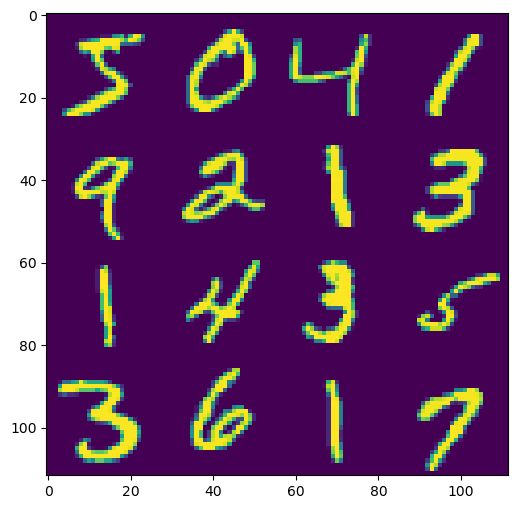
This is a large dataset with many features against which we can train or use algorithms.
Student Performance#
The student performance dataset is a synthetic dataset that included student performance (the dependent variable) based on a range of independent variables, including both continuous and discrete values.
data = pd.read_csv('../data/student-performance.csv')
data
| Hours Studied | Previous Scores | Extracurricular Activities | Sleep Hours | Sample Question Papers Practiced | Performance Index | |
|---|---|---|---|---|---|---|
| 0 | 7 | 99 | Yes | 9 | 1 | 91.0 |
| 1 | 4 | 82 | No | 4 | 2 | 65.0 |
| 2 | 8 | 51 | Yes | 7 | 2 | 45.0 |
| 3 | 5 | 52 | Yes | 5 | 2 | 36.0 |
| 4 | 7 | 75 | No | 8 | 5 | 66.0 |
| ... | ... | ... | ... | ... | ... | ... |
| 9995 | 1 | 49 | Yes | 4 | 2 | 23.0 |
| 9996 | 7 | 64 | Yes | 8 | 5 | 58.0 |
| 9997 | 6 | 83 | Yes | 8 | 5 | 74.0 |
| 9998 | 9 | 97 | Yes | 7 | 0 | 95.0 |
| 9999 | 7 | 74 | No | 8 | 1 | 64.0 |
10000 rows × 6 columns
We will use this data to understand regression approaches, where we try to describe trends in data.