Multiple Linear Regression#
The matrix implementation of linear regression discussed previously naturally extends to data with more than one feature. For example, let’s look at applying to the student performance dataset.
import pandas as pd

data = pd.read_csv('../data/student-performance.csv')
data
| Hours Studied | Previous Scores | Extracurricular Activities | Sleep Hours | Sample Question Papers Practiced | Performance Index | |
|---|---|---|---|---|---|---|
| 0 | 7 | 99 | Yes | 9 | 1 | 91.0 |
| 1 | 4 | 82 | No | 4 | 2 | 65.0 |
| 2 | 8 | 51 | Yes | 7 | 2 | 45.0 |
| 3 | 5 | 52 | Yes | 5 | 2 | 36.0 |
| 4 | 7 | 75 | No | 8 | 5 | 66.0 |
| ... | ... | ... | ... | ... | ... | ... |
| 9995 | 1 | 49 | Yes | 4 | 2 | 23.0 |
| 9996 | 7 | 64 | Yes | 8 | 5 | 58.0 |
| 9997 | 6 | 83 | Yes | 8 | 5 | 74.0 |
| 9998 | 9 | 97 | Yes | 7 | 0 | 95.0 |
| 9999 | 7 | 74 | No | 8 | 1 | 64.0 |
10000 rows × 6 columns
You will notice that the Extracurricular Activities is a discrete variable, either Yes or No. We must encode this as an integer to work with linear regression.
data['Encoded EA'] = [1 if x == 'Yes' else 0 for x in data['Extracurricular Activities']]
To assess the success of the linear regressor, we will split the data using a now familiar process.
from sklearn.model_selection import train_test_split

train, test = train_test_split(data, test_size=0.2, random_state=42)
We will produce the \(\mathbf{X}\) matrix from the training set. We achieve this by adding the column of ones to our independent variables.
import numpy as np

X = np.hstack([np.ones((train.shape[0], 1)),
               train.drop(['Performance Index', 'Extracurricular Activities'], axis=1).values])
We see five features in the dataset, and by using multiple linear regression, we can feed these all into the prediction. The outcome that we are assessing is the Performance Index.
y = train['Performance Index'].values
Then, we use the normal equations to estimate \(\beta\).
import numpy as np

beta = np.linalg.inv(X.T @ X) @ X.T @ y
beta
array([-33.92194622,   2.85248393,   1.0169882 ,   0.47694148,
         0.19183144,   0.60861668])
So, we now understand the power that each feature has on the data. Note that it would be necessary to normalise our data to conclude these \(\beta\) values. However, here, we are interested in the ability of the model to predict new performance based on our features. We can compute the estimated Performance Index using this multiple linear regression.
X_test = np.hstack([np.ones((test.shape[0], 1)),
                    test.drop(['Performance Index', 'Extracurricular Activities'], axis=1).values])

y_est = X_test @ beta
We can visualise the accuracy of this approach with a predicted versus actual plot, where the dashed line indicates perfect estimation.
import matplotlib.pyplot as plt

fig, ax = plt.subplots()
ax.plot(y_est, test['Performance Index'], '.')
ax.plot([0, 100], [0, 100], 'k--')
ax.set_xlabel('Predicted')
ax.set_ylabel('Actual')
ax.set_aspect('equal')
plt.show()
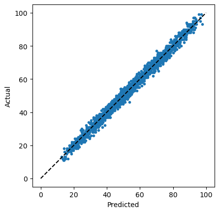
This provides a good visual indication of the accuracy of the linear regression. However, we can also calculate metrics, such as the mean-squared error (MSE).
from sklearn.metrics import mean_squared_error

mean_squared_error(test['Performance Index'], y_est)
4.082628398521898
This metric is computed as the mean of the square of the difference between the estimated and the true value,