Linear Regression

Linear regression is a fundamental data analysis component and the backbone of modern machine-learning approaches. Linear regression is modelling a linear relationship between two parameters, the dependent and independent variables. For example, consider the following data measuring the heart rate of patients while they are walking/running on an elliptical machine.

import pandas as pd
import matplotlib.pyplot as plt

data = pd.read_csv('../data/heart-rate.csv')

fig, ax = plt.subplots()
data.plot(x='speed (kph)', y='heart rate (bpm)', kind='scatter', ax=ax)
plt.show()

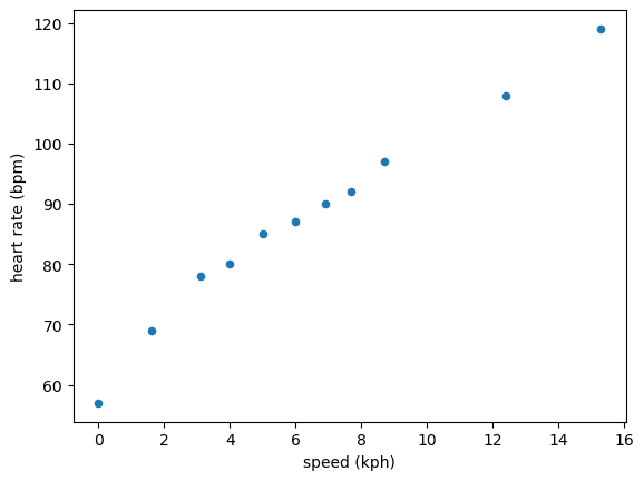
The data appears to be linear. Therefore, it is a good use of linear regression to describe the trend in the data. The aim of linear regression is to find the parameters \(\beta\) that solve the following equation,

\[ \mathbf{X}\beta = \mathbf{y}, \]

where, \(\mathbf{y}\) is a column vector containing \(n\) independent variables, \(\mathbf{X}\) is a \(n\times p\) matrix, where \(p\) is the number of features in the data, and \(\mathbf{\beta}\) is another column vector of length \(p\). \(\beta\) will describe each feature’s impact on the data.

Considering the simple linear regression case, two parameters must be determined: the slope and the intercept. Therefore, \(\mathbf{X}\) will have two columns; the first column will be a column where all the elements have the value 1, and the second will be the dependent variables. So for the heart rate data previously, the \(\mathbf{X}\) matrix would be

(35)\[\begin{split} \mathbf{X} = \begin{bmatrix} 1 & 0 \\ 1 & 1.6 \\ 1 & 3.1 \\ 1 & 4.0 \\ 1 & 5.0 \\ 1 & 6.0 \\ 1 & 6.9 \\ 1 & 7.7 \\ 1 & 8.7 \\ 1 & 12.4 \\ 1 & 15.3 \end{bmatrix}. \end{split}\]

This matrix can be generated as a NumPy array.

import numpy as np

x = data['speed (kph)']
X = np.array([np.ones_like(x), x]).T
X.shape

(11, 2)

The \(\mathbf{y}\) vector will then be the dependent variable.

y = data['heart rate (bpm)'].T
y

0      57
1      69
2      78
3      80
4      85
5      87
6      90
7      92
8      97
9     108
10    119
Name: heart rate (bpm), dtype: int64

Once again, the estimates of the slope and intercept, \(\hat{\mathbf{\beta}}\), are found by minimising the sum of squared differences between \(\mathbf{X}\mathbf{\beta}\) and \(\mathbf{y}\), which can be referred to as \(S(\mathbf{\beta})\). This gives rise to what is known as the normal equations:

(36)\[ (\mathbf{X}^\top\mathbf{X})\hat{\mathbf{\beta}} = \mathbf{X}^\top\mathbf{y}. \]

The normal equations can be rearranged to give \(\hat{\mathbf{\beta}}\),

Note

This matrix multiplication function may be familiar.

(37)\[ \hat{\mathbf{\beta}} = (\mathbf{X}^\top\mathbf{X})^{-1}\mathbf{X}^\top\mathbf{y}. \]

This allows us to write the following NumPy matrix mathematics.

beta = np.linalg.inv(X.T @ X) @ X.T @ y
beta

array([63.35675743,  3.74930224])

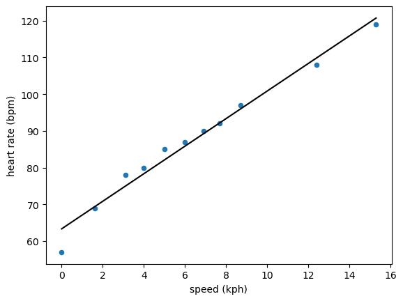
This tells us that the intercept, linked to the column of ones, is 63.36 bpm, and the gradient is 3.75 bpm/kph. We can use this to plot this linear trend alongside the data.

fig, ax = plt.subplots()
data.plot(x='speed (kph)', y='heart rate (bpm)', kind='scatter', ax=ax)
ax.plot(x, X @ beta, 'k-')
plt.show()

Note

You may notice that to obtain the straight line of best fit in the plot above, the code X @ beta is used. This is the matrix implementation of \(y = m x + c\).

The scikit-learn way

Another method that can be used to perform the same operation is available in the scikit-learn package, a Python package focusing on machine learning tools. The approach of using scikit-learn is slightly different because scikit-learn methods typically follow a machine learning “training” approach. First, a LinearRegression() object is created.

from sklearn.linear_model import LinearRegression

model = LinearRegression()

Then, to get our data in a form that the LinearRegression object can ingest, it is necessary to withdraw the NumPy arrays from the pandas.DataFrame and then “reshape” the arrays. This reshaping ensures that the arrays are two-dimensional, which is the expected dimensionality for scikit-learn.

x = data['speed (kph)'].to_numpy().reshape(-1, 1)
y = data['heart rate (bpm)'].to_numpy().reshape(-1, 1)

Note

Fitting is not a good term for this, as no numerical optimisation occurs in linear regression. As will be seen later, fitting is only necessary for non-linear analysis.

The “fitting” is then done by passing the reshaped independent and dependent variances to the fit method for the LinearRegression object.

model.fit(x, y)

LinearRegression()

In a Jupyter environment, please rerun this cell to show the HTML representation or trust the notebook.
On GitHub, the HTML representation is unable to render, please try loading this page with nbviewer.org.

The different regression parameters can then be obtained as the model attributes. For example, the slope is coef_ (short for coefficients), and the intercept is intercept_.

model.coef_, model.intercept_

(array([[3.74930224]]), array([63.35675743]))

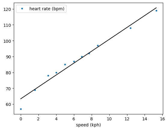
scikit-learn provides a convenience function for producing the line of best fit over a given set of x-values, predict. This means that the plot can be produced, as shown below.

fig, ax = plt.subplots()
data.plot(x='speed (kph)', y='heart rate (bpm)', marker='.', linestyle='', ax=ax)
ax.plot(data['speed (kph)'], model.predict(x), 'k-')
plt.show()

You may notice that the slope and intercept are the same for both methods. This is because linear regression has a definite result, i.e., no random fitting procedure is involved; therefore, the same result will always be found for the same input data.