A Toy Example

To show logistic regression in practice, we will use a toy problem, specifically the data shown below.

import pandas as pd
import matplotlib.pyplot as plt
import seaborn as sns

data = pd.read_csv("../data/toy.csv")

fix, ax = plt.subplots()
sns.scatterplot(x='x', y='y', data=data, hue='label', ax=ax)
plt.show()

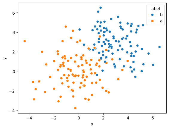
This data is two-dimensional, with an x and y-dimension. Each data point is labelled as either a or b. Clearly, b-points generally have larger values in both x and y. Therefore, it should be straightforward to produce a classification algorithm for this.

However, the labels are not currently computer-readable, and to use the logistic function described previously, we need to encode them as 1s and 0s. Below, we add this encoding to the pandas DataFrame.

Note

This can also be achieved with a pandas apply method using a lambda function. You can find information online on how to achieve this.

data['encoded_label'] = [1 if i == 'b' else 0 for i in data['label'].values]
data

	x	y	label	encoded_label
0	2.091675	5.076054	b	1
1	1.670044	1.893883	b	1
2	-3.473584	-1.836446	a	0
3	2.418901	2.087297	b	1
4	2.028405	2.998328	b	1
...	...	...	...	...
195	-0.103211	2.971752	a	0
196	-0.484741	-0.347390	a	0
197	1.624884	3.894923	b	1
198	2.874282	0.696651	b	1
199	4.710780	4.261925	b	1

200 rows × 4 columns

Splitting the Data

Since we are applying this to a supervised machine learning approach, splitting the data into training and testing data is good practice. The training data is used to develop the model, where the weights and bias are optimised. The testing data is used to check that the model is well generalised and can be applied to data it has not seen before. We can use the sklearn.model_selection.train_test_split method to separate the data.

from sklearn.model_selection import train_test_split

train, test = train_test_split(data, test_size=0.2, random_state=0)

fig, ax = plt.subplots(1, 2, figsize=(10, 4), sharex=True, sharey=True)
sns.scatterplot(x='x', y='y', data=train, hue='label', ax=ax[0])
sns.scatterplot(x='x', y='y', data=test, hue='label', ax=ax[1])
ax[0].set_title('Training Data')
ax[1].set_title('Testing Data')
plt.show()

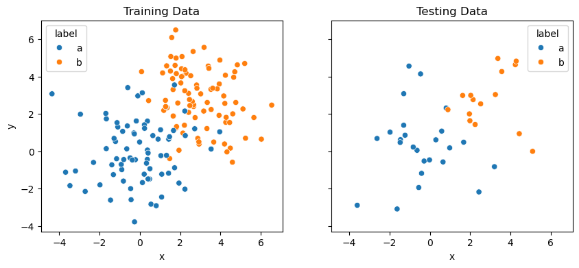
Above, we kept 20 % of the data for testing and will use 80 % for training.

Training

To perform the training/optimisation, we will write our own implementation of the gradient descent algorithm. To do this, let’s take advantage of the JAX library and the built-in automatic differentiation that it enables. To start, we will turn all necessary values into jnp.array objects.

import jax.numpy as jnp

X = jnp.array(train[['x', 'y']].values)
y = jnp.array(train['encoded_label'].values)

Next, we will create random values for the weights and bias.

from jax import random

key = random.PRNGKey(0)
weights = random.normal(key, (2))
bias = random.normal(key, (1))
weights, bias

(Array([-0.78476596,  0.85644484], dtype=float32),
 Array([-0.20584226], dtype=float32))

Now, we create the function that is to be optimised. This is achieved by bringing together the parts discussed previously. Below, we define a single function that encapsulates the calculation of the loss function that we are looking to optimise.

from jax.lax import logistic

def to_optimise(weights, bias):
    z = jnp.dot(X, weights) + bias
    f = logistic(z)
    L = -1 * jnp.mean((y * jnp.log(f) + (1 - y) * jnp.log(1 - f)))
    return L

Using JAX, we can find the first derivative easily.

from jax import grad

first_order = grad(to_optimise)

Finally, we implement the gradient descent algorithm where the step size is the learning rate.

learning_rate = 0.01

result = first_order(weights, bias)

for i in range(2000):
    weights = weights - learning_rate * result[:-1]
    bias = bias - learning_rate * result[-1]
    result = first_order(weights, bias)

We run this for 2000 iterations, with a learning rate of 0.01. These are the hyperparameters of our logistic regression function. We can now see the values for the weights and bias.

weights, bias

(Array([1.055286 , 2.6964939], dtype=float32),
 Array([-4.274763], dtype=float32))

These values can then be used to classify the training dataset, and we can see how good the model is for the data it has already seen.

import numpy as np

z = np.dot(train[['x', 'y']], weights) + bias
f = logistic(z)
prediction = np.array(['nd'] * len(f))
prediction[np.where(f > 0.5)] = 'b'
prediction[np.where(f <= 0.5)] = 'a'
train['prediction'] = prediction

This has added a now column to our DataFrame.

train

	x	y	label	encoded_label	prediction
134	0.373930	1.619907	a	0	b
66	2.294891	4.181484	b	1	b
26	0.432925	2.717288	b	1	b
113	1.355748	2.339877	b	1	b
168	1.423604	-1.171737	a	0	a
...	...	...	...	...	...
67	1.941346	0.058802	b	1	a
192	2.237253	-2.026433	a	0	a
117	1.516596	4.297617	b	1	b
47	2.230459	2.158100	a	0	b
172	0.327218	-0.634313	a	0	a

160 rows × 5 columns

Here, we use the accuracy_score, a percentage of how many times the predicted label was correct, to quantify how well the model is doing.

from sklearn.metrics import accuracy_score

accuracy_score(train['label'], train['prediction'])

0.90625

The current model is correct around 90.6 % of the time on the training data. But how does it work for data it has never seen before?

z = np.dot(test[['x', 'y']], weights) + bias
f = logistic(z)
prediction = np.array(['x'] * len(f))
prediction[np.where(f > 0.5)] = 'b'
prediction[np.where(f <= 0.5)] = 'a'
test['prediction'] = prediction

accuracy_score(test['label'], test['prediction'])

0.9

Impressively, it is better for the data it has not yet seen.

By plotting just the predictions, we can see one of the problems with the logistic regression approach.

fig, ax = plt.subplots(1, 2, figsize=(10, 4), sharex=True, sharey=True)
sns.scatterplot(x='x', y='y', data=train, hue='prediction', ax=ax[0])
sns.scatterplot(x='x', y='y', data=test, hue='prediction', ax=ax[1])
ax[0].set_title('Training Data')
ax[1].set_title('Testing Data')
plt.show()

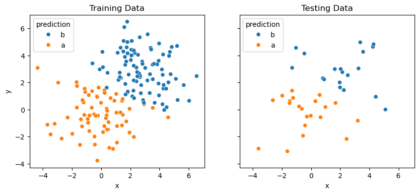
It is clear that there is a linear discrimination between the classes a and b. This means that logistic regression would be potentially ineffective where the classification of the data does not follow a linear trend. Strictly speaking, handling non-linear relationships with logistic regression requires feature engineering. This is where the features are adapted to improve linear discrimination between classes.