Eigenthings

If we consider the non-zero vector, \(\mathbf{v} = \begin{bmatrix} 1 \\ 1 \end{bmatrix}\), shown in Fig. 16. There is a matrix \(\mathbf{A}\) that describes a linear transformation of \(\mathbf{v}\) to \(\mathbf{v'}\), which scales the vector by a scaler, \(\lambda\) (in Fig. 16, \(\lambda=3\)). We can write this as a matrix-vector multiplication \(\mathbf{A}\mathbf{v} = \mathbf{v'}\), which can be generalised as:

(25)\[ \mathbf{A}\mathbf{v} = \lambda\mathbf{v}. \]

Note

The prefix eigen- is adopted from the German word eigen, meaning ‘proper’, ‘characteristic’, or ‘own’.

\(\mathbf{v}\) is an eigenvector of the linear transformation \(\mathbf{A}\), while \(\lambda\) is the corresponding eigenvalue.

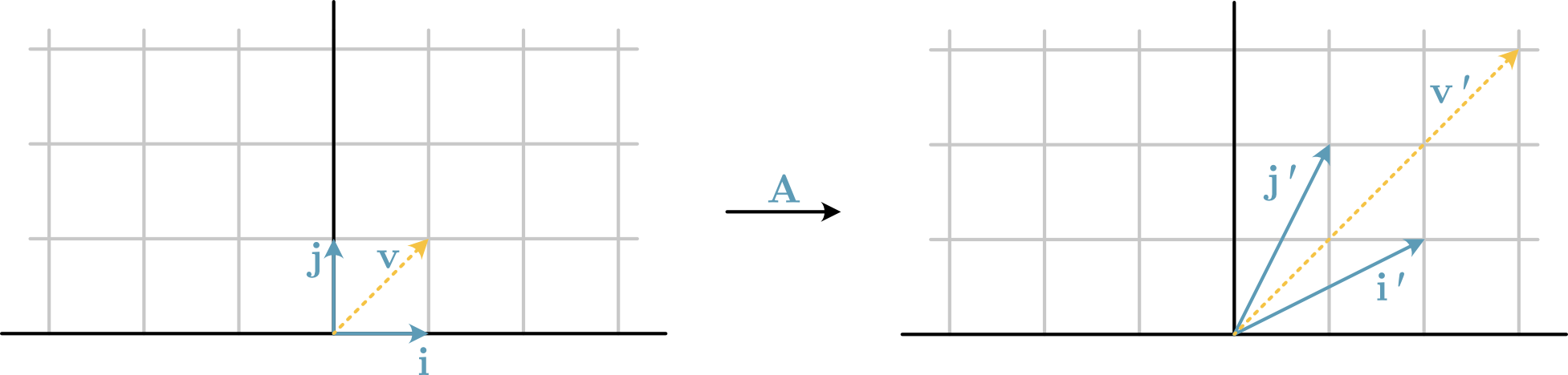
Fig. 16 A linear transformation is described by the matrix \(\mathbf{A}\), which is an eigenfunction of the vector \(\mathbf{v}\).

Eigenvalues and eigenvectors have broad applicability across science and engineering; therefore, we will see them come up a few times in this course book. The application that is most familiar to those with a physics or chemistry background is probably in the Schrödinger equation. Though, eigenvalues and eigenvectors also play an important role in data analysis approaches, such as principal components analysis.

Finding the Eigenvalues and Eigenvectors of a Matrix

For many applications, the matrix is known and we want to find the relevant eigenvalues and eigenvectors. Consider, for example, the time-independent Schrödinger equation, which is used to calculate the energy of the wavefunction some quantum mechanical systems, has the form,

\[ H \psi_E = E \psi_E, \]

where, \(H\) is the Hamiltonian matrix, \(\psi_E\) is the wavefunction and \(E\) is the energy. It is clear that this has the same form, as Eqn. (25), where \(\psi_E\) is the eigenvector and \(E\) is the eigenvalue. Therefore, being able to calculate the eigenvalues and eigenvectors of the Hamiltonian matrix would give us the energy and wavefunction of our system.

For a square-matrix the solution to find the eigenvalues and eigenvectors can be considered as a rearrangement of Eqn. (25), followed by finding the roots of a quadratic equation. Firstly, both sides of Eqn. (25) are multiplied by an identity matrix, \(\mathbf{I}\) of the same shape as \(\mathbf{A}\),

\[ \mathbf{A}\mathbf{I}\mathbf{v} = \lambda\mathbf{I}\mathbf{v}. \]

Any matrix multiplied by an identity matrix, is just the original matrix, i.e., \(\mathbf{A}\mathbf{I} = \mathbf{A}\). Therefore, we can write

\[ \mathbf{A}\mathbf{v} = \lambda\mathbf{I}\mathbf{v}, \]

rearrange,

\[ \mathbf{A}\mathbf{v} - \lambda\mathbf{I}\mathbf{v} = 0, \]

and take \(\mathbf{v}\) out as a common factor,

\[ (\mathbf{A} - \lambda\mathbf{I})\mathbf{v} = 0. \]

Then, for any non-zero vector \(\mathbf{v}\),

(26)\[ |\mathbf{A} - \lambda\mathbf{I}| = 0, \]

which is to say that the determinant of \(\mathbf{A} - \lambda\mathbf{I}\) is equal to 0. To show this second step, it is easiest to use an example. Consider the matrix \(\mathbf{A}\) that describes the linear transformation shown in Fig. 16,

\[\begin{split} \mathbf{A} = \begin{bmatrix} 2 & 1 \\ 1 & 2 \end{bmatrix}. \end{split}\]

We write this in the form of Eqn. (26),

\[\begin{split} \text{det} \left(\begin{bmatrix} 2 & 1 \\ 1 & 2 \end{bmatrix} - \begin{bmatrix} \lambda & 0 \\ 0 & \lambda \end{bmatrix}\right) = 0. \end{split}\]

Therefore,

\[\begin{split} \text{det} \left(\begin{bmatrix} 2 - \lambda & 1 \\ 1 & 2 - \lambda \end{bmatrix}\right) = 0, \end{split}\]

and calculating the determinant, using \(ad - bc\),

\[ (2 - \lambda)(2 - \lambda) - 1\times 1 = 3 - 4\lambda + \lambda^2 = (\lambda - 3)(\lambda - 1) = 0, \]

returns the eigenvalues of \(\lambda = 3\) and \(\lambda = 1\). Then to find the eigenvector for \(\lambda = 3\), we find the solution to \((\mathbf{A} - 3\mathbf{I})\mathbf{v} = 0\),

\[\begin{split} \left(\begin{bmatrix} 2 & 1 \\ 1 & 2 \end{bmatrix} - \begin{bmatrix} 3 & 0 \\ 0 & 3 \end{bmatrix}\right) \begin{bmatrix} v_1 \\ v_2 \end{bmatrix} = \begin{bmatrix} -1 & 1 \\ 1 & -1 \end{bmatrix} \begin{bmatrix} v_1 \\ v_2 \end{bmatrix} = \begin{bmatrix} 0 \\ 0 \end{bmatrix}. \end{split}\]

We can expand these matrix multiplications for clarity, so,

\[\begin{split} \begin{aligned} -v_1 + v_2 & = 0 \\ v_1 - v_2 & = 0. \end{aligned} \end{split}\]

These two conditions can hold true for any vector where \(v_1\) and \(v_2\) are equal, i.e., \(\mathbf{v}\) in Fig. 16. The second eigenvector for the matrix \(\mathbf{A}\) is found by substituting \(\lambda = 1\).

\[\begin{split} \left(\begin{bmatrix} 2 & 1 \\ 1 & 2 \end{bmatrix} - \begin{bmatrix} 1 & 0 \\ 0 & 1 \end{bmatrix}\right) \begin{bmatrix} v_1 \\ v_2 \end{bmatrix} = \begin{bmatrix} 1 & 1 \\ 1 & 1 \end{bmatrix} \begin{bmatrix} v_1 \\ v_2 \end{bmatrix} = \begin{bmatrix} 0 \\ 0 \end{bmatrix}. \end{split}\]

Again, for clarity, we expand the matrix multiplication,

\[\begin{split} \begin{aligned} v_1 + v_2 & = 0 \\ v_1 + v_2 & = 0, \end{aligned} \end{split}\]

which can only hold true for vectors where \(v_1 = -v_2\).

Eigenvalues and Eigenvectors with NumPy

Naturally, NumPy can be used to find the eigenvalues and eigenvectors of a given matrix. We achieve this with the np.linalg.eig function. Let’s use this to check the results of the mathematics above.

import numpy as np

A = np.array([[2, 1], [1, 2]])
eigenthings = np.linalg.eig(A)
print(eigenthings.eigenvalues)

[3. 1.]

We can see that the same eigenvalues were determined.

print(eigenthings.eigenvectors)

[[ 0.70710678 -0.70710678]
 [ 0.70710678  0.70710678]]

The eigenvectors are a little more complex to parse. If we look at the documentation for the np.linalg.eig function, it can help us to understand, specifically the following text:

eigenvectors: The normalized (unit “length”) eigenvectors, such that the column eigenvectors[:,i] is the eigenvector corresponding to the eigenvalue eigenvalues[i].

So the columns of the eigenthings.eigenvectors are the normalised eigenvectors for each eigenvalue. This also agrees with what we have shown above.

Eigendecomposition

Any square diagonalizable matrix can be broken down into a set of simpler components. This is known as eigendecomposition and, as we shall see, has significant utility in science and engineering.

Note

Diagonalizable in this context means that an \(nxn\) matrix has a complete set of \(n\) independent eigenvectors. Any matrix with non independent eigenvectors is not diagonizable and, therefore, cannot be decomposed via eigendecomposition.

The eigendecomposition of the matrix \(\mathbf{A}\) is expressed as:

(27)\[ \mathbf{A} = \mathbf{Q}\mathbf{\Lambda}\mathbf{Q}^{-1}, \]

where \(\mathbf{Q}\) is a matrix whose columns are the eigenvectors of \(\mathbf{A}\) and \(\mathbf{\Lambda}\) is a diagonal matrix whose diagonal entries are the eigenvalues of \(\mathbf{A}\). Therefore, using the eigendecomposition logic, we should be able to reconstruct \(\mathbf{A}\) from these constituent parts.

Q = eigenthings.eigenvectors
Lambda = np.diag(eigenthings.eigenvalues)
Q @ Lambda @ np.linalg.inv(Q)

array([[2., 1.],
       [1., 2.]])