Optimisation#
Optimisation is an important concept when we consider the application of computation and mathematics to the physical sciences. A common goal in chemistry and physics is to find the configuration of atoms that minimises the energy of some system. This is typically achieved computationally through some optimisation algorithm. This algorithm will iteratively propose new configurations of atoms until that with the minimum energy is found.
Minimisation vs Maximisation
Optimisation algorithms may be used to minimise some function (in the example above, the system’s energy is the function) or maximise a function (for example, it can be desirable to maximise some probability distribution). For all intents and purposes, when it comes to optimisation, these are equivalent. You can convince yourself of this by considering a maximisation of some function as the minimisation of its negative. Indeed, this is practically how this is often achieved.
Naturally, the most straightforward approach to finding the minimum of some function would be:
Select a range of values for which to compute the function.
Evenly distribute \(n\) points on that grid.
Compute the function for these points.
Find the point where the function is smallest. However, there are apparent issues with this algorithm, in particular that increasing the number of dimensions (variables) in your problem increases the computation exponentially. Instead, let’s look at some algorithms that are smarter in terms of the approach they take.
Gradient Descent Method#
The gradient descent method, also known as the steepest descent, can be thought of as following the path of a ball down a hill. The ball will find the bottom of the hill (the minimum of our function) if we let it roll long enough (perform enough iterations of the algorithm). This is achieved by computing the gradient of the function we want to minimise using differentiation. Let’s look now at the algorithm, consider trying to find the value of \(x\) that optimises the function \(f(x)\):
Starting with some initial guess for \(x\).
Calculate the gradient \(\frac{\text{d}f(x)}{x}\), at \(x\).
Change the value of \(x\) so that the value of \(f(x)\) decreases, i.e., change \(x\) by some amount \(\Delta x\) in the direction opposite to the gradient.
Repeat 2 and 3 until the gradient is close to zero.
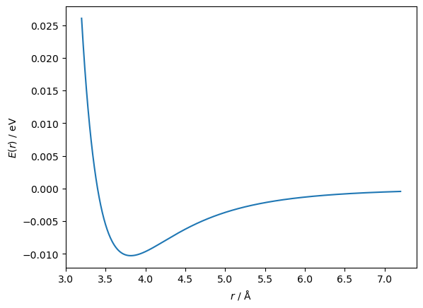
For example, let’s consider the minimisation (optimisation) of a classical function from computational chemistry/physics, known as the Lennard-Jones potential. This function has the following form,
where, \(A\) and \(B\) are system specific coefficients and \(r\) is the distance between two atoms. Below, we plot a Lennard-Jones potential commonly used to model argon atoms [1].
import matplotlib.pyplot as plt
import numpy as np

def lennard_jones(r, A, B):
    """
    Computes the first derivative of the Lennard-Jones
    potential.

    :param r: Distance between atoms
    :param A: First coefficient.
    :param B: Second coefficient.

    :returns: First derivative of Lennard-Jones at r.
    """
    return A / r ** 12 - B / r ** 6

A = 98320.5
B = 63.6
r = np.linspace(3.2, 7.2, 1000)

fig, ax = plt.subplots()

ax.plot(r, lennard_jones(r, A, B))
ax.set_xlabel('$r$ / Å')
ax.set_ylabel('$E(r)$ / eV')
plt.show()
We can then use sympy to find the derivative.
from sympy import symbols, diff

r_, A_, B_ = symbols('r A B')
lj = A_ / r_ ** 12 - B_ / r_ ** 6
diff(lj, r_)
We can then use this to define a function that computes the derivative.
def first_derivative(r, A, B):
    """
    Computes the first derivative of the Lennard-Jones
    potential.

    :param r: Distance between atoms
    :param A: First coefficient.
    :param B: Second coefficient.

    :returns: First derivative of Lennard-Jones at r.
    """
    return -12 * A / r ** 13 + 6 * B / r ** 7
We can then put a simple gradient descent algorithm together as follows.
n_iterations = 1000
initial_r = 5
delta_r = 0.02

r_values = np.array([initial_r])
for i in range(n_iterations):
    first = first_derivative(r_values[-1], A, B)
    if np.isclose(np.abs(first), 0):
        break
    r_values = np.append(r_values, r_values[-1] - np.sign(first) * delta_r)
Above, the algorithm can run for 1000 iterations, but if the first derivative is very small, close to zero, we stop early.
We can see how many iterations have run by looking at the length of the r_values array.
len(r_values)
1001
So it took all 1001 steps, indicating that it may not have found the minimum. Let’s have a look at the results.
r_values[-10:]
array([3.82, 3.8 , 3.82, 3.8 , 3.82, 3.8 , 3.82, 3.8 , 3.82, 3.8 ])
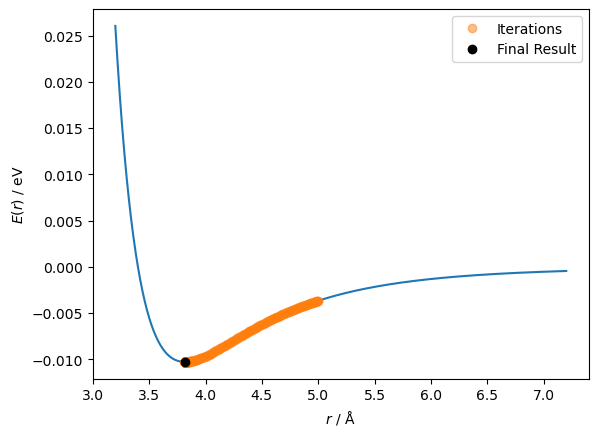
We can see that the last ten values iterated through were moving back and forth between 3.80 and 3.82 Å. This is because the minimum is somewhere between these two values, and the step size is 0.02 Å. We can visualise this path on the function.
fig, ax = plt.subplots()

ax.plot(r, lennard_jones(r, A, B))
ax.plot(r_values[:-1], lennard_jones(r_values[:-1], A, B), 'o', alpha=0.5, label='Iterations')
ax.plot(r_values[-1], lennard_jones(r_values[-1], A, B), 'ko', label='Final Result')
ax.set_xlabel('$r$ / Å')
ax.set_ylabel('$E(r)$ / eV')
ax.legend()
plt.show()

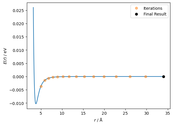
The gradient descent algorithm clearly has a very important hyperparameter, the step size \(\Delta x\). This hyperparameter defines how long the algorithm will take to reach the minimum. There is a slight improvement that is commonly used, where the gradient is used to scale the step size, i.e., instead of just using the gradient’s sign. This will mean that the step size will be smaller when the gradient is close to 0.
n_iterations = 1000
initial_r = 5
delta_r = 1.5

r_values = np.array([initial_r])
for i in range(n_iterations):
    first = first_derivative(r_values[-1], A, B)
    if np.isclose(np.abs(first), 0):
        break
    r_values = np.append(r_values, r_values[-1] - first * delta_r)
len(r_values)
298
This time, a solution was found in just 298 steps. So the improvement worked!
fig, ax = plt.subplots()

ax.plot(r, lennard_jones(r, A, B))
ax.plot(r_values[:-1], lennard_jones(r_values[:-1], A, B), 'o', alpha=0.5, label='Iterations')
ax.plot(r_values[-1], lennard_jones(r_values[-1], A, B), 'ko', label='Final Result')
ax.set_xlabel('$r$ / Å')
ax.set_ylabel('$E(r)$ / eV')
ax.legend()
plt.show()
It is clear that we can find the minimum more easily with this scaled step size. However, a hyperparameter is still present. Can we adapt this algorithm to remove the hyperparameter?
The Newton-Raphson Method#
An adaptation which does not require any hyperparameters is known as the Newton-Raphson method. The adaption involves changing the function that updates \(x\), which is now,
where \(f'(x_{\text{old}})\) and \(f''(x_{\text{old}})\) are the first and second derivatives at \(x_{\text{old}}\) of the function being optimised. To update the algorithm above with this new update function, we need the second derivative of the Lennard-Jones function.
diff(lj, r_, r_)
def second_derivative(r, A, B):
    """
    Computes the second derivative of the Lennard-Jones
    potential.

    :param r: Distance between atoms
    :param A: First coefficient.
    :param B: Second coefficient.

    :returns: First derivative of Lennard-Jones at r.
    """
    return 6 * (26 * A / r ** 6 - 7 * B) / r ** 8
With the second derivative, we can now implement the algorithm.
n_iterations = 1000
initial_r = 4

r_values = np.array([initial_r])
for i in range(n_iterations):
    first = first_derivative(r_values[-1], A, B)
    second = second_derivative(r_values[-1], A, B)
    if np.abs(first) < 5e-12:
        break
    r_values = np.append(r_values, r_values[-1] - first / second)

fig, ax = plt.subplots()

ax.plot(r, lennard_jones(r, A, B))
ax.plot(r_values[:-1], lennard_jones(r_values[:-1], A, B), 'o', alpha=0.5, label='Iterations')
ax.plot(r_values[-1], lennard_jones(r_values[-1], A, B), 'ko', label='Final Result')
ax.set_xlabel('$r$ / Å')
ax.set_ylabel('$E(r)$ / eV')
ax.legend()
plt.show()
len(r_values)
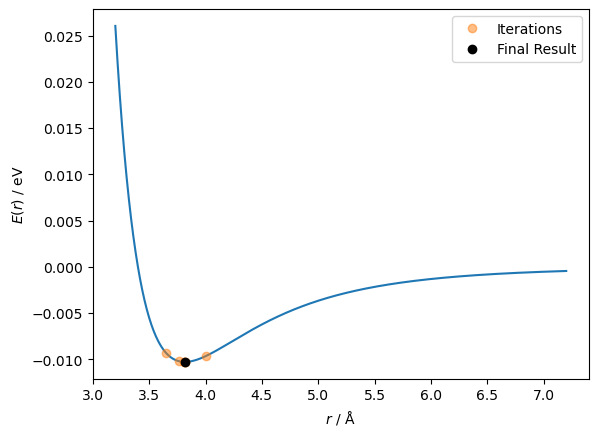
7
This time, the algorithm only took seven steps to reach the minimum, but you may notice that the initial guess was 4 Å instead of the 5 Å that was used previously. This is due to the Newton-Raphson method’s drawback, which we can understand by plotting the second derivative.
fig, ax = plt.subplots()

r_tight = np.linspace(4, 5, 100)

ax.plot(r_tight, second_derivative(r_tight, A, B))
ax.axhline(0, color='k', ls='--')
ax.set_xlabel('$r$ / Å')
ax.set_ylabel("$E''(r)$ / eV Å$^{-2}$")
plt.show()
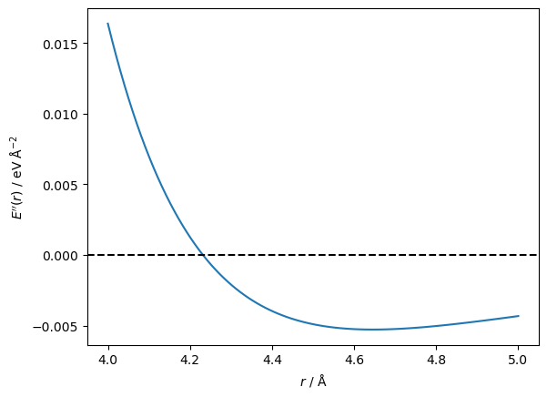
The second derivative goes from positive to negative at a distance between particles of around 4.2 Å. The first derivative has moved through a stationary point at this value. Furthermore, the Newton-Raphson method will try to move the particles further apart rather than closer together. Let’s see that in action.
n_iterations = 1000
initial_r = 5

r_values = np.array([initial_r])
for i in range(n_iterations):
    first = first_derivative(r_values[-1], A, B)
    second = second_derivative(r_values[-1], A, B)
    if np.isclose(np.abs(first), 0):
        break
    r_values = np.append(r_values, r_values[-1] - first / second)

r_wide = np.linspace(r.min(), r_values.max(), 1000)

fig, ax = plt.subplots()

ax.plot(r_wide, lennard_jones(r_wide, A, B))
ax.plot(r_values[:-1], lennard_jones(r_values[:-1], A, B), 'o', alpha=0.5, label='Iterations')
ax.plot(r_values[-1], lennard_jones(r_values[-1], A, B), 'ko', label='Final Result')
ax.set_xlabel('$r$ / Å')
ax.set_ylabel('$E(r)$ / eV')
ax.legend()
plt.show()
This indicates the importance of a good starting point in running some optimisation algorithms.
These two algorithms are just the start of a journey that has become a whole field of mathematics. We won’t look at more complex gradient descent style algorithms in detail, but many build on the principles outlined here.
scipy.optimize.minimize#
The scipy package implements a vast range of minimisation algorithms.
These cover various problems, such as constraints or bounds in the variables.
The minimize function can dynamically select an appropriate algorithm for the problem, at hand.
Let’s look at how we can use it.
from scipy.optimize import minimize

res = minimize(lennard_jones, x0=[5], args=(A, B))
We can see that the minimize function takes a few arguments; the first is the function to minimise, the second x0 is the initial guess of the parameters and args is the non-variable parameters that should be passed to the function being minimised.
A range of other keyword arguments can be found in the documentation.
The minimize function returns a special type called an OptimizeResult; let’s look at the contents.
res
  message: Optimization terminated successfully.
  success: True
   status: 0
      fun: -0.01028513890791614
        x: [ 3.817e+00]
      nit: 4
      jac: [ 6.647e-08]
 hess_inv: [[ 1.978e+01]]
     nfev: 26
     njev: 13
The most important information are:
success: This indicates whether the optimisation was successful.x: The optimised value of the parameter(s).nit: The number of iterations.
We can see that the algorithm selected by scipy.optimize.minimize was able to find the solution in just four iterations.
So far, we have focused on optimisation problems where there is only one local minimum, the global minimum. However, many problems in science have many local minima that we want to avoid to find the global solution. We will look at some global optimisation approaches later.