Thinking About Data Probabilistically#
No measurement is 100 % accurate, therefore, in many scientific applications there is uncertainty associated with our data. Including this uncertainty in the modelling and analysis we do is of paramount important as it can effect the certainty that we have about our conclusions. This section will look at some examples of probabilistic and Bayesian modelling.
Let’s consider the following data file to help us think about our data in a slightly different way.
import pandas as pd

data = pd.read_csv('../data/first-order.csv')
data
| t | At | At_err | |
|---|---|---|---|
| 0 | 2 | 6.23 | 0.3 |
| 1 | 6 | 3.76 | 0.3 |
| 2 | 10 | 2.60 | 0.3 |
| 3 | 14 | 1.85 | 0.3 |
| 4 | 18 | 1.27 | 0.3 |
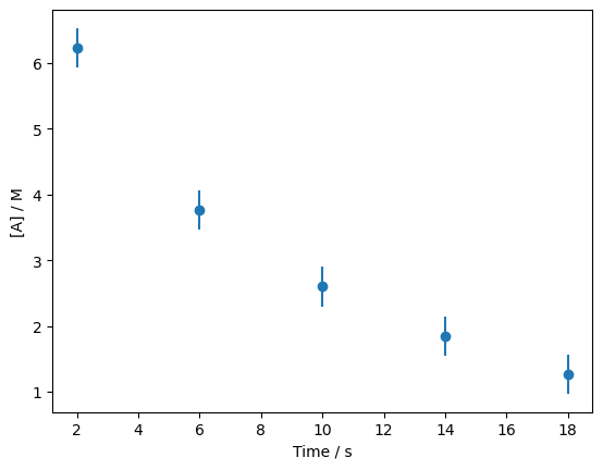
This data is measurements of the concentration of a chemical species as a function of time, when it is undergoing a reaction. This data was from a chemistry textbook [4]. There are three columns, the first is the time, the second is the concentration and the third is the error in the concentration. Plotting data such as this with error bars is common, like we do below.
import matplotlib.pyplot as plt

fig, ax = plt.subplots()
ax.errorbar(data['t'], data['At'], data['At_err'], fmt='o')
ax.set_xlabel('Time / s')
ax.set_ylabel('[A] / M')
plt.show()
The Meaning of Error Bars#
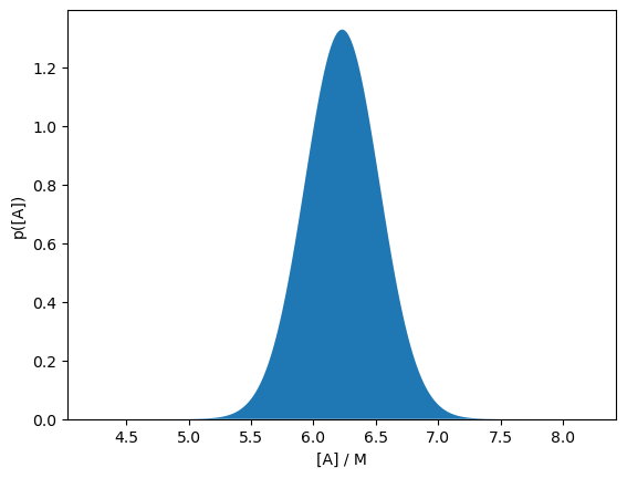
The meaning of error bars are often overlooked. What specifically are we describing with these vertical lines? Well, the answer is, that depends. The error bar often describes a single standard deviation, as the measurement is assumed to be normally distributed. Therefore, if we take the data point at 2 seconds and imagine we are sitting on the plot looking down the x-axis, it would look like this.
import numpy as np
from scipy.stats import norm

a_range = np.linspace(data['At'][0] - 2, data['At'][0] + 2, 1000)

fig, ax = plt.subplots()

ax.fill_between(a_range, norm.pdf(a_range, data['At'][0], data['At_err'][0]))
ax.set_xlabel('[A] / M')
ax.set_ylabel('p([A])')
ax.set_ylim(0, None)
plt.show()
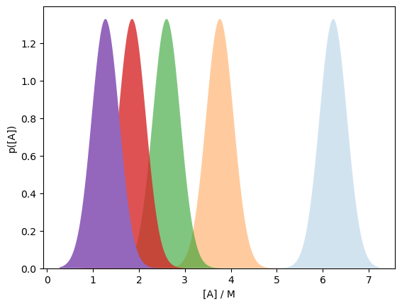
Indeed, we could take this further and plot all five probability distributions in this way.
a_range = np.linspace(data['At'].min() - 1, data['At'].max() + 1, 1000)

fig, ax = plt.subplots()
[ax.fill_between(a_range,
                 norm.pdf(a_range, data['At'][i], data['At_err'][i]),
                 alpha=(i+1) / len(data))
                 for i in range(len(data))]
ax.set_xlabel('[A] / M')
ax.set_ylabel('p([A])')
ax.set_ylim(0, None)
plt.show()
Data Aren’t Always Normal
Be aware, that our data will not always be normally distributed, however, by treating our data probabilistically, as we will see, we can handle data following any distribution. Despite this, it is rare for experimentally collected data to be treated as anything but normal – there are various reasons for this. Still, the most important is that random noise leads to a normal distribution, due to the central limit theorem.